Stat 435 Lecture Notes 2a
Xiongzhi Chen
Washington State University

Inference on coefficients
Inference on estimates
Since the observations \((x_i,y_i),i=1,\ldots,n\) for \((X,Y)\) are random, so is the LSE \(\left(\hat{\beta}_0,\hat{\beta}_1\right)\).
\(\left(\hat{\beta}_0,\hat{\beta}_1\right)\) is unbiased, i.e., \(E(\hat{\beta}_0)=\beta_0\) and \(E(\hat{\beta}_1)=\beta_1\), when \(\varepsilon_i\)’s are uncorrelated
How accurate is \(\left(\hat{\beta}_0,\hat{\beta}_1\right)\) with respect to \(({\beta}_0,{\beta}_1)\)?
Variability of estimates
Recall \[\hat{\beta}_1 = \frac{\sum (x_i - \bar{x})(y_i - \bar{y})}{\sum (x_i - \bar{x})^2}\] and \(\hat{\beta}_0 = \bar{y} - \hat{\beta}_1 \bar{x}\).
When \(\varepsilon_i\)’s are uncorrelated,
- \([SE(\hat{\beta_0})]^2 = \sigma^2 \left[\frac{1}{n}+\frac{\bar{x}^2}{\sum_{i=1}^n(x_i - {\bar{x}})^2}\right]\)
- \([SE(\hat{\beta_1})]^2 = \frac{\sigma^2}{\sum_{i=1}^n(x_i - \bar{x})^2}\)
How does the sample size \(n\) and the sample variance of \(x_i\)’s affect these variances?
Variability of estimates
Variances of \(\hat{\beta_0}\) and \(\hat{\beta_1}\) contain information on the accuracy of \(\hat{\beta}_0\) and \(\hat{\beta}_1\)
Without information on \(\sigma\), variances of \(\hat{\beta_0}\) and \(\hat{\beta_1}\) cannot be accurately assessed
An estimate of \(\sigma\) is
\[RSE = \sqrt{RSS/(n-2)} = \sqrt{\frac{\sum_{i=1}^n (y_i - \hat{y}_i)^2}{n-2}}\]
CI for estimates
The approximate \(95\%\) confidence interval (CI)
- for \(\hat{\beta_0}\) is \(\hat{\beta_0} \pm 2 \cdot SE(\hat{\beta_0})\)
- for \(\hat{\beta_1}\) is \(\hat{\beta_1} \pm 2 \cdot SE(\hat{\beta_1})\)
Note: the above follows a general principle for constructing a CI when the distribution of “estimate minus parameter” is symmetric around \(0\)
Testing the slope
- Recall the model \[Y = \beta_0 + \beta_1 X + \varepsilon\] with \(E(\varepsilon)=0\) and \(Var(\varepsilon)=\sigma^2\)
- If \(\beta_1=0\), then \(Y = \beta_0 + \varepsilon\), and \(Y\) is independent of \(X\) (when \(\varepsilon\) is independent \(X\)).
- Testing “\(H_0: \beta_1=0\)” often is equivalent to checking if “\(H_0\): there is no relationship between \(X\) and \(Y\)”.
Caution: The random error \(\varepsilon\) may not be independent of \(X\) and \(Y\) due to latent dependence, which is common in genetics studies.
Testing the slope
- A test statistic for this purpose is the t-statistic \[t = \frac{\hat{\beta}_1 - 0}{SE(\hat{\beta}_1)}\]
- If \(SE(\hat{\beta}_1)\) is small, then relatively small \(\vert \hat{\beta}_1\vert\) provides strong evidence that \(\beta_1 \ne 0\)
Note: When \(H_0: \beta_1=0\) holds, \(t\) approximately has a \(t\)-distribution with \(n-2\) degrees of freedom when \(\varepsilon_i\)’s are not much dependent on each other; when \(n\) is large, a \(t\)-distribution will be close to a Gaussian distribution.
Testing the slope
Model: \(E\)(sales) = \(\beta_0\) + \(\beta_1\) TV:
# A tibble: 2 x 5
  term        estimate std.error statistic  p.value
  <chr>          <dbl>     <dbl>     <dbl>    <dbl>
1 (Intercept)   7.03     0.458        15.4 1.41e-35
2 TV 0.0475 0.00269 17.7 1.47e-42- Is \(H_0: \beta_1=0\) retained or rejected? In either case, at which Type I error level?
- How trustable are our conclusions?
Testing the slope
Model \(E\)(mpg) = \(\beta_0\) + \(\beta_1\) horsepower:
# A tibble: 2 x 5
  term        estimate std.error statistic   p.value
  <chr>          <dbl>     <dbl>     <dbl>     <dbl>
1 (Intercept)   39.9     0.717        55.7 1.22e-187
2 horsepower -0.158 0.00645 -24.5 7.03e- 81- Is \(H_0: \beta_1=0\) retained or rejected? In either case, at which Type I error level?
- How trustable are our conclusions?
Model diagnostics
Things to check
- Nonlinearity of relationship between response and predictor
- Correlation of error terms
- Non-constant variance of error terms
- Outliers
- High-leverage points
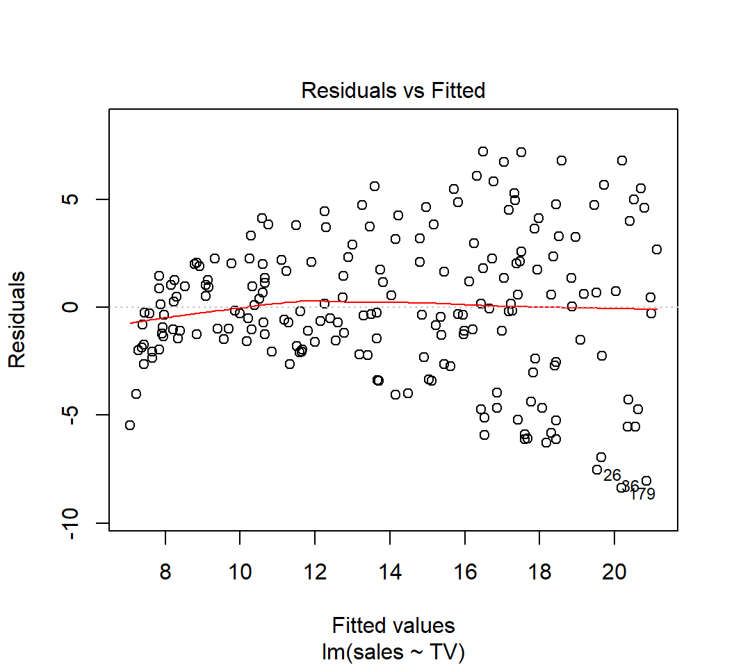
Nonlinearity
If the linear model \[Y=\beta_0 + \beta_1 X + \varepsilon\] is plausible, then
- \(y_i = \beta_0 + \beta_1 x_i + \varepsilon_i\), where \(\varepsilon_i\) is a realization of \(\varepsilon\) for each pair \((x_i,y_i)\)
- the residuals \(e_i\)’s, where \[e_i = y_i - \hat{y}_i, \quad \hat{y}_i=\hat{\beta}_0 + \hat{\beta}_1 x_i,\] are random errors (as estimated realizations from \(\varepsilon\)), and should have no specific relationship with \(x_i\)’s
So, the residuals \(e_i\)’s should contain no specific pattern on the fitted values \(\hat{y}_i\)’s or \(x_i\)’s if the model is plausible.
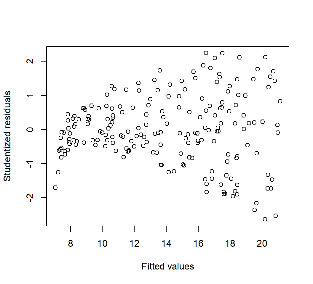
Nonlinearity
Model: \(E\)(sales) = \(\beta_0\) + \(\beta_1\) TV:
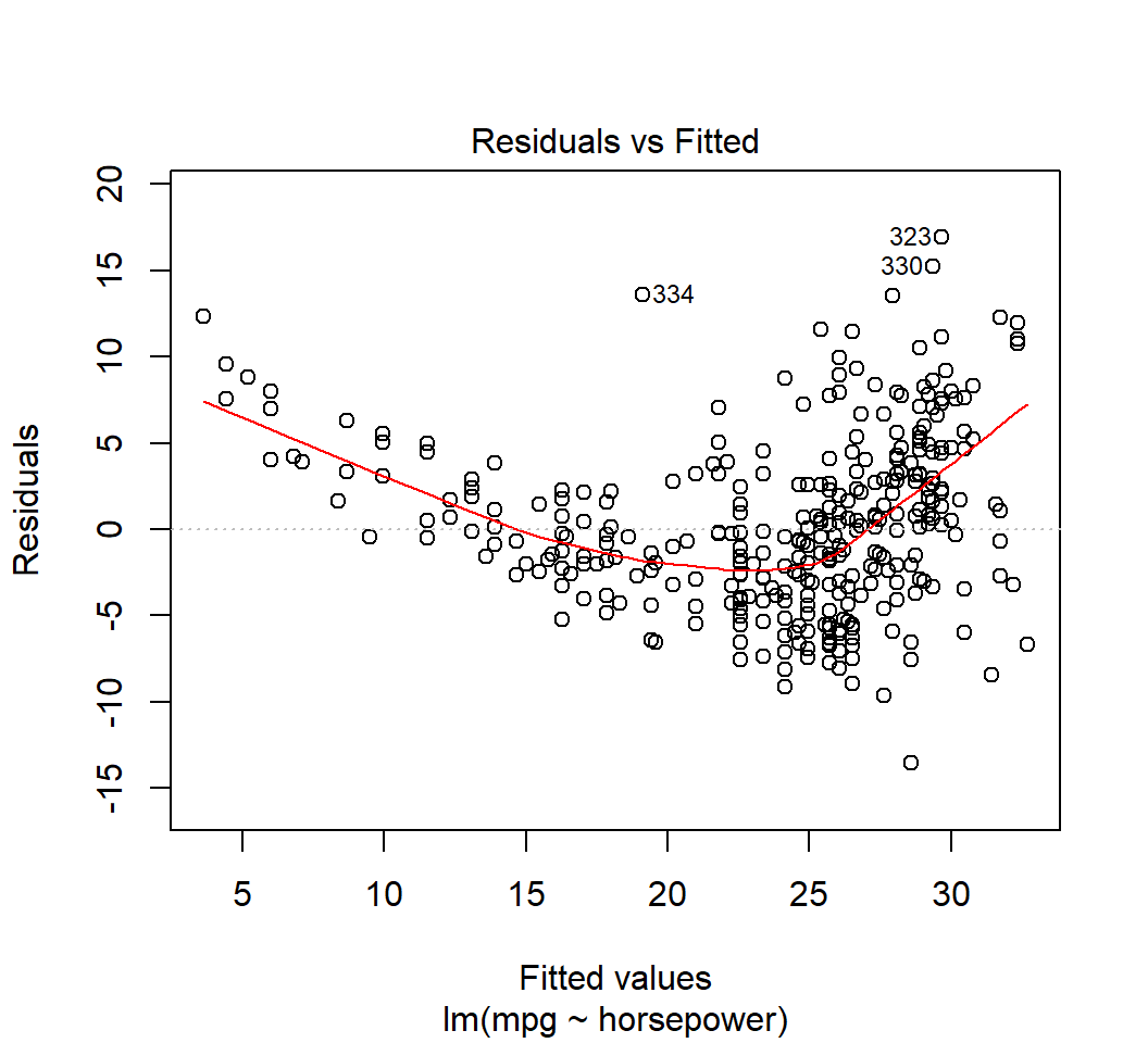
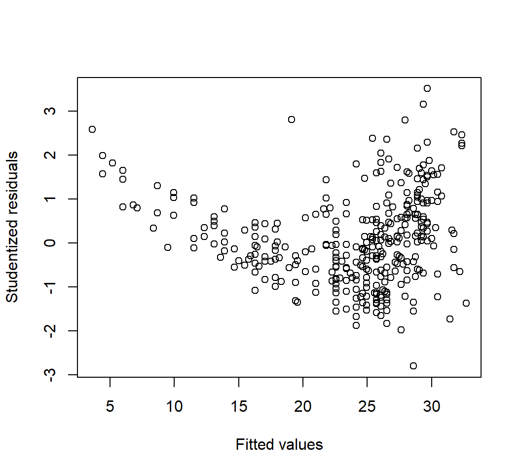
Nonlinearity
Model \(E\)(mpg) = \(\beta_0\) + \(\beta_1\) horsepower:
Check on error terms
- Inference on the LSE \((\hat{\beta_0}, \hat{\beta_1})\) depends critically on \(SE(\hat{\beta_0})\) and \(SE(\hat{\beta_1})\), which depend on the unknown \(\sigma = \sqrt{Var(\varepsilon)}\).
- Information on \(\varepsilon\), hence on \(\sigma\), is contained in the residuals \(e_i\) (as estimates of \(\varepsilon_i\))
Relatively accurate inference requires \(e_i\)’s to
- be uncorrelated
- have identical variance
Otherwise, the formulae for \(SE(\hat{\beta_0})\) and \(SE(\hat{\beta_1})\) are (usually) invalid, leading to invalid inference.
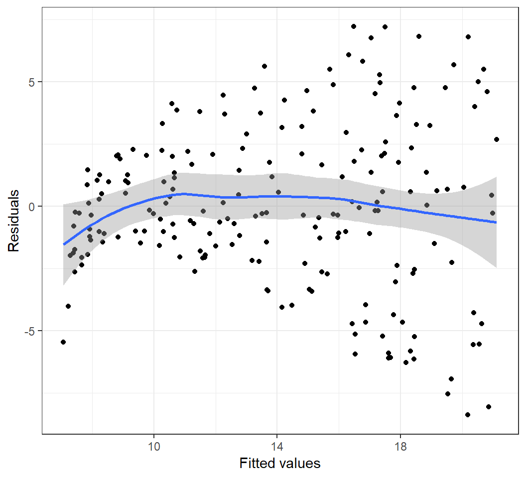
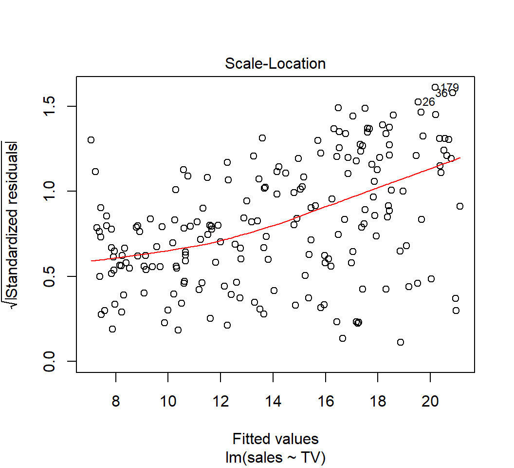
Heterogeneous error variances
Model: \(E\)(sales) = \(\beta_0\) + \(\beta_1\) TV:
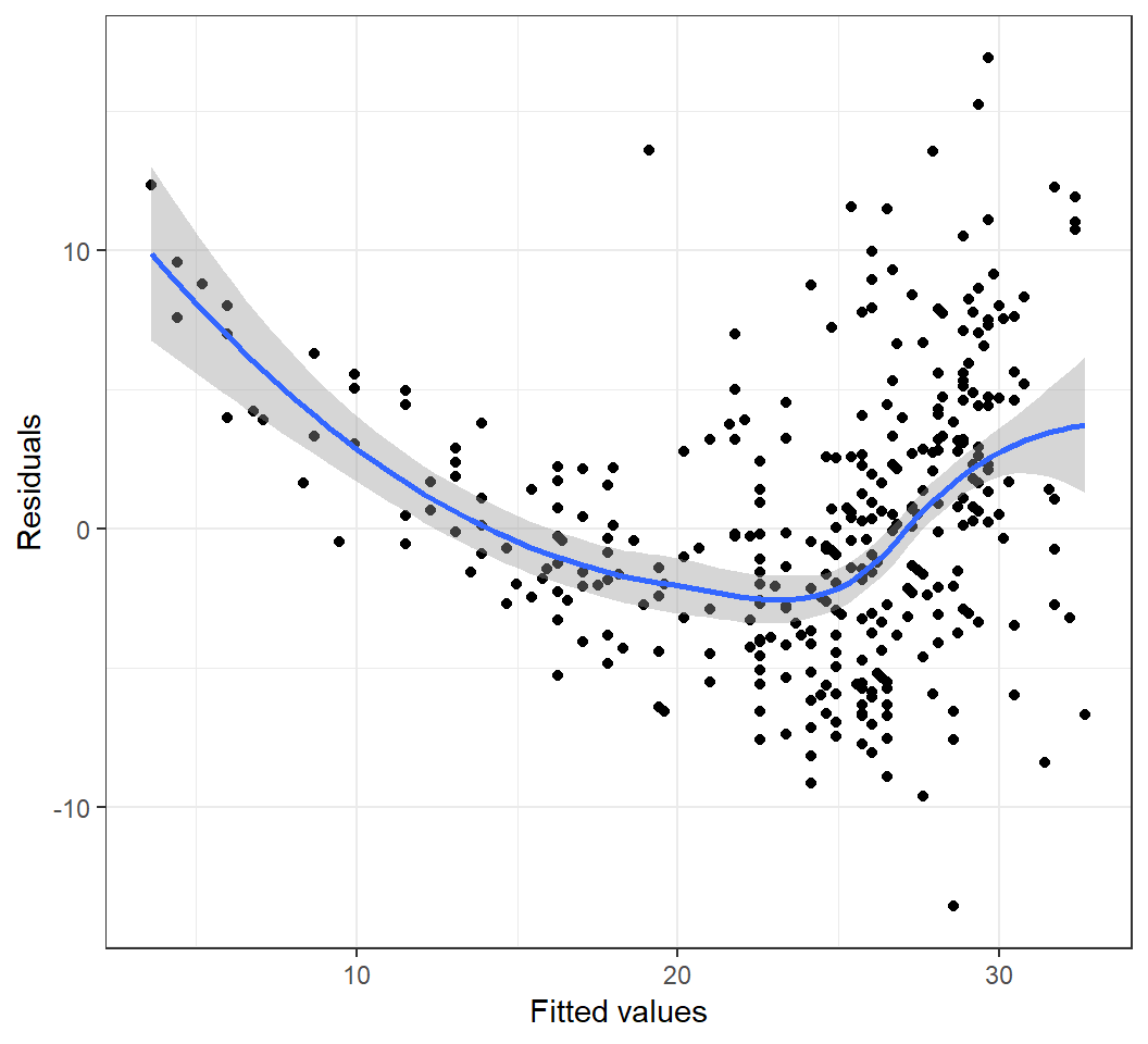
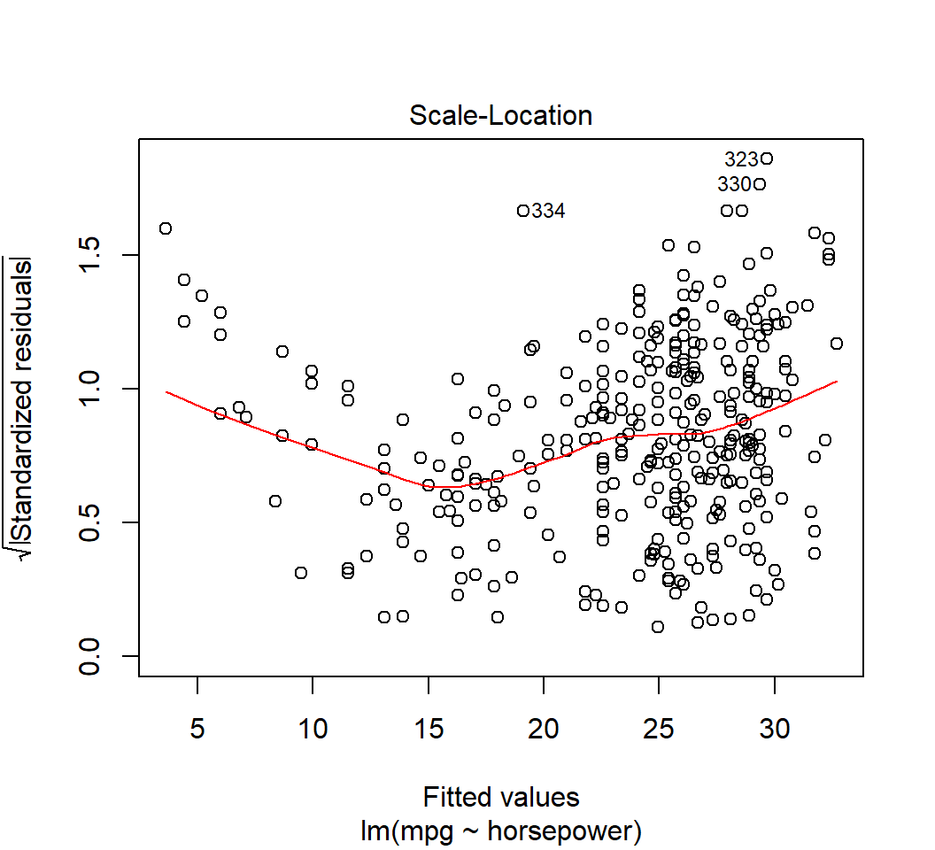
Heterogeneous error variances
Model \(E\)(mpg) = \(\beta_0\) + \(\beta_1\) horsepower:
Outliers
- An outlier is an observation \((x_i,y_i)\) for which \(y_i\) is far from the value predicted by the model
- Observations whose studentized residuals are greater than \(3\) in absolute value are possible outliers
- An outlier may significantly affect RSE (i.e., residual standard error) and \(R^2\)
- Removing an outlier may or may not significantly affect the subsequent estimated regression line, and this is related to high-leverage points
Outliers
Model: \(E\)(sales) = \(\beta_0\) + \(\beta_1\) TV:
Outliers
Model: \(E\)(sales) = \(\beta_0\) + \(\beta_1\) TV:
Outliers
Model \(E\)(mpg) = \(\beta_0\) + \(\beta_1\) horsepower:
Outliers
Model \(E\)(mpg) = \(\beta_0\) + \(\beta_1\) horsepower:
High-leverage points
- A high-leverage point is an observation \((x_i,y_i)\) for which \(x_i\) is unusual among all observations for \(X\)
- Removing a high-leverage point often significantly affects the subsequent estimated regression line
- Let \(p\) be the number of predictors in the model and \(n\) the sample size, if the leverage statistic for an observation greatly exceeds \((p+1)/n\), then it can be considered a high-leverage point
High-leverage points
Model: \(E\)(sales) = \(\beta_0\) + \(\beta_1\) TV (\(p=1\),\(n=397\), \(\tilde{h}=(p+1)/n \approx 0.005\)): 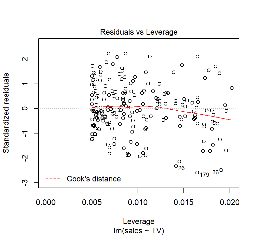
High-leverage points
Model \(E\)(mpg) = \(\beta_0\) + \(\beta_1\) horsepower (\(p=1\),\(n=200\),\(\tilde{h}=(p+1)/n=0.01\)): 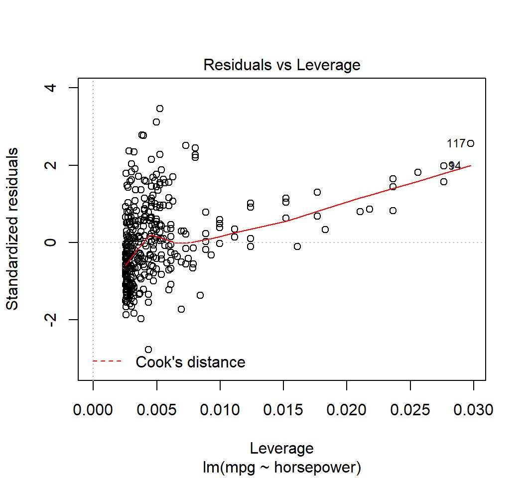
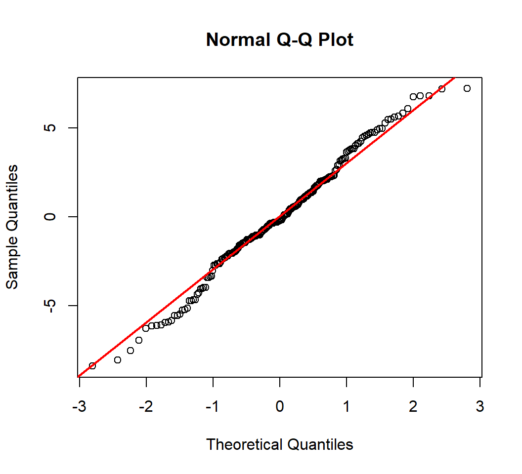
Q-Q Plot
A Q-Q (quantile-quantile) plot plots observed quantiles against the quantiles of a theoretical distribution, and hence provides information on whether observations under investigation have a distribution that matches this theoretical distribution
- A normal Q-Q plot does this with the standard Normal distribution as the theoretical distribution
- In a normal Q-Q plot, x-axis plots the theoretical quantiles from the standard Normal distribution with mean 0 and standard deviation 1
Test on Normality
- Model: \(E\)(
sales) = \(\beta_0\) + \(\beta_1\)TV - Test Normality of random error
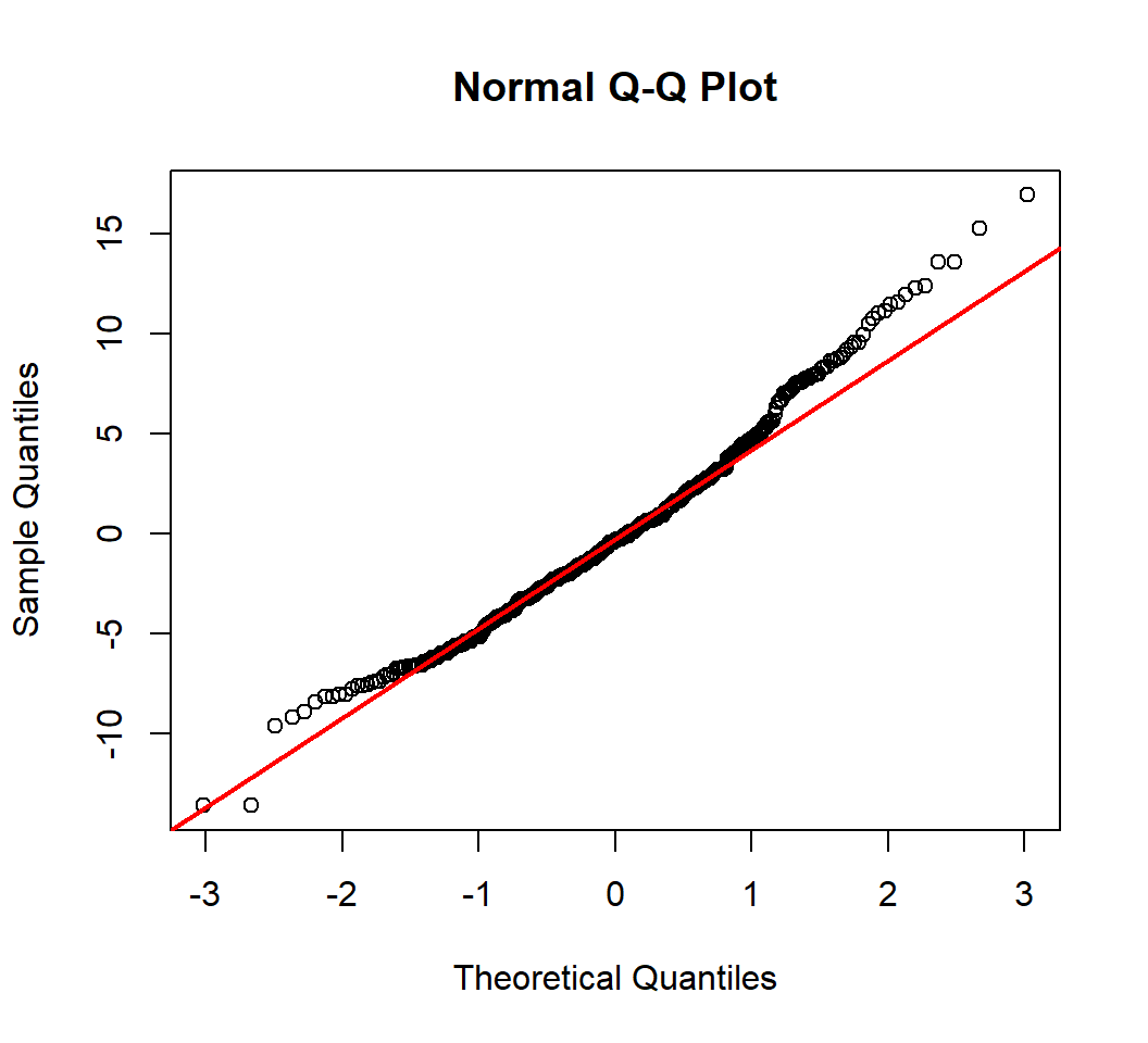
Test on Normality
- Model \(E\)(
mpg) = \(\beta_0\) + \(\beta_1\)horsepower - Test Normality of random error
Kolmogorov-Smirnov Test
- Model: \(E\)(
sales) = \(\beta_0\) + \(\beta_1\)TV Fit1is the object obtained from fitting the model- Test Normality of random error
    One-sample Kolmogorov-Smirnov test

data:  Fit1$residuals
D = 0.041533, p-value = 0.8806
alternative hypothesis: two-sided
Kolmogorov-Smirnov Test
- Model \(E\)(
mpg) = \(\beta_0\) + \(\beta_1\)horsepower Fit2is the object obtained from fitting the model- Test Normality of random error
    One-sample Kolmogorov-Smirnov test

data:  Fit2$residuals
D = 0.060525, p-value = 0.1131
alternative hypothesis: two-sided
Correlation of error terms
It is extremely important that the error terms are uncorrelated. Correlated error terms often present in time series data and in data with latent variables. Such correlation affects
- testing if random errors are Normally distributed
- variances of estimated coefficients and variance of random error term
- Testing independence is a highly nontrival issue in statistical learning
Correlation of error terms
The true model is \[Y = 1 + 2X + \varepsilon\] with \(n=1000\) observations \[y_{i} = 1+ 2 x_{i} + \varepsilon_{i}\]
The random errors are equally correlated, such that \[\varepsilon_{i} = \sqrt{1-0.3}X_{i} + \sqrt{0.3} X_{0}\] and \(X_{0}, X_{1}, \ldots, X_{1000}\) are i.i.d. standard Normal.
Fit a simple linear model and obtain fitted values and residuals
Correlation of error terms
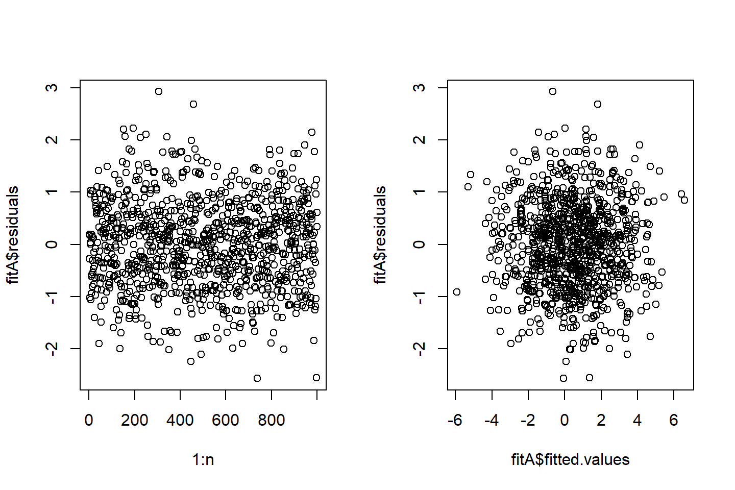
Correlation of error terms
For this example, when trying to check if the random errors are independent or uncorrelated by a visual check, we see the following:
- no pattern in the left plot where each residuals is plotted against its index
- the random errors are dependent, since if they were independent, the fitted values should be independent of the residuals
- the random errors do not seem to be correlated with the fitted values
Appendix
True model
For two quantitative random variables \(Y\) and \(X\), a simple linear model is \[E(Y) = \beta_0 + \beta_1 X,\] where \(\beta_0\) (intercept) and \(\beta_1\) (slope) are unknown, true model parameters (or coefficients), and \(\beta_1\) is called the regression coefficient.
The above model is equivalent to \[Y = \beta_0 + \beta_1 X + \varepsilon \quad \text{ with } \quad E(\varepsilon)=0,Var(\varepsilon)=\sigma^2\] which is called the population regression line.
The least squares estimate
With observations \((x_i,y_i),i=1,\ldots,n\) for \((X,Y)\), the LS method gives the least squares estimate (LSE):
\(\hat{\beta}_1 = \frac{\sum (x_i - \bar{x})(y_i - \bar{y})}{\sum (x_i - \bar{x})^2}\) with \(\bar{y}=n^{-1}\sum_{i=1}^n y_i\)
\(\hat{\beta}_0 = \bar{y} - \hat{\beta}_1 \bar{x}\) with \(\bar{x}=n^{-1}\sum_{i=1}^n x_i\)
Namely, the fitted model is \[\hat{y} = \hat{\beta}_0 + \hat{\beta}_1 x,\] also called the least squares line.
License and session Information
> sessionInfo()
R version 3.5.0 (2018-04-23)
Platform: x86_64-w64-mingw32/x64 (64-bit)
Running under: Windows 10 x64 (build 19041)

Matrix products: default

locale:
[1] LC_COLLATE=English_United States.1252
[2] LC_CTYPE=English_United States.1252
[3] LC_MONETARY=English_United States.1252
[4] LC_NUMERIC=C
[5] LC_TIME=English_United States.1252

attached base packages:
[1] stats     graphics  grDevices utils     datasets  methods
[7] base

other attached packages:
[1] ggplot2_3.1.0 broom_0.5.1   knitr_1.21

loaded via a namespace (and not attached):
 [1] Rcpp_1.0.3       plyr_1.8.4       pillar_1.3.1
 [4] compiler_3.5.0   tools_3.5.0      digest_0.6.18
 [7] evaluate_0.12    tibble_2.1.3     nlme_3.1-137
[10] gtable_0.2.0     lattice_0.20-35  pkgconfig_2.0.2
[13] rlang_0.4.4      cli_1.0.1        rstudioapi_0.8
[16] yaml_2.2.0       xfun_0.4         withr_2.1.2
[19] dplyr_0.8.4      stringr_1.3.1    generics_0.0.2
[22] revealjs_0.9     grid_3.5.0       tidyselect_0.2.5
[25] glue_1.3.0       R6_2.3.0         fansi_0.4.0
[28] rmarkdown_1.11   purrr_0.2.5      tidyr_0.8.2
[31] magrittr_1.5     backports_1.1.3  scales_1.0.0
[34] htmltools_0.3.6  assertthat_0.2.0 colorspace_1.3-2
[37] labeling_0.3     utf8_1.1.4       stringi_1.2.4
[40] lazyeval_0.2.1   munsell_0.5.0    crayon_1.3.4