Motivation

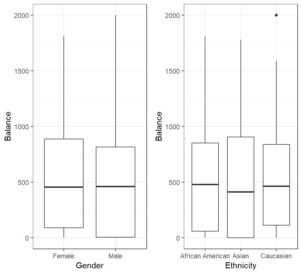
• How is Balance of a credit card related to a user’s Gender?

• How is Balance of a credit card related to a user’s Ethnicity?

Motivation

Model 1: 2 levels

• Coding: Gender has 2 levels, Male and Female
• dummy variable: \(x_i =0\) if \(i\)th person is Female and \(x_i =1\) if \(i\)th person is Male
• Model: \(y_i = \beta_0 + \beta_1 x_i + \varepsilon_i\), which induces 2 submodels:
• \(y_i = \beta_0 + \beta_1 + \varepsilon_i\) if \(i\)th person is Male
• \(y_i = \beta_0 + \varepsilon_i\) if \(i\)th person is Female

Note: dummy variable follows coding by R, for which the first level Female is the baseline

Model 1: 2 levels

Model: \(y_i = \beta_0 + \beta_1 x_i + \varepsilon_i\)

• \(x_i =0\) if \(i\)th person is Female, and \(x_i =1\) if \(i\)th person is Male
• \(\beta_0\): average Balance for females
• \(\beta_1\): average difference in balance between males and females

Remark: coding of a dummy variable is arbitrary and should be easily interpretable

Fitting the Model 1

Call:
lm(formula = Balance ~ Gender, data = creditData)

Coefficients:
(Intercept)   GenderMale  
     529.54       -19.73  

• Females have an average balance of $529.54; Female baseline
• Males have an average balance of $(529.54-19.73)= $509.80

Note: in R, by default the first level Female is the baseline

Testing the Model 1

Call:
lm(formula = Balance ~ Gender, data = creditData)

Residuals:
    Min      1Q  Median      3Q     Max 
-529.54 -455.35  -60.17  334.71 1489.20 

Coefficients:
            Estimate Std. Error t value Pr(>|t|)    
(Intercept)   529.54      31.99  16.554   <2e-16 ***
GenderMale    -19.73      46.05  -0.429    0.669    
---
Signif. codes:  0 '***' 0.001 '**' 0.01 '*' 0.05 '.' 0.1 ' ' 1

Residual standard error: 460.2 on 398 degrees of freedom
Multiple R-squared:  0.0004611, Adjusted R-squared:  -0.00205 
F-statistic: 0.1836 on 1 and 398 DF,  p-value: 0.6685

• If model assumptions are met, Gender is not significant on affecting average balance at type I error level 0.05 based on F-statistic (or the p-value of GenderMale)

Model 2: 3 levels

Ethnicity has 3 levels African American (1st level and baseline in R), Asian, and Caucasian. 2 dummy variables are needed:

• \(x_{i1} =0\) if \(i\)th person is not Asian, and \(x_{i1} =1\) if \(i\)th person is Asian
• \(x_{i2} =0\) if \(i\)th person is not Caucasian, and \(x_{i2} =1\) if \(i\)th person is Caucasian
• Model: \[y_i = \beta_0 + \beta_1 x_{i1} +\beta_2 x_{i2} + \varepsilon_i\]

Model 2: 3 levels

Model: \[y_i = \beta_0 + \beta_1 x_{i1} +\beta_2 x_{i2} + \varepsilon_i\]

• Codings on previous slide
• \(\beta_0\): average balance for African American
• \(\beta_1\): average difference in balance between Asian and African American
• \(\beta_2\): average difference in balance between Caucasian and African American

Fitting the Model 2

Call:
lm(formula = Balance ~ Ethnicity, data = creditData)

Coefficients:
       (Intercept)      EthnicityAsian  EthnicityCaucasian  
            531.00              -18.69              -12.50  

• African Americans have an average balance of $531
• Asians have an average balance of $(531-18.69)= $512.31
• Caucasians have an average balance of $(531-12.50)= $518.5

Testing the Model 2

Call:
lm(formula = Balance ~ Ethnicity, data = creditData)

Residuals:
    Min      1Q  Median      3Q     Max 
-531.00 -457.08  -63.25  339.25 1480.50 

Coefficients:
                   Estimate Std. Error t value Pr(>|t|)    
(Intercept)          531.00      46.32  11.464   <2e-16 ***
EthnicityAsian       -18.69      65.02  -0.287    0.774    
EthnicityCaucasian   -12.50      56.68  -0.221    0.826    
---
Signif. codes:  0 '***' 0.001 '**' 0.01 '*' 0.05 '.' 0.1 ' ' 1

Residual standard error: 460.9 on 397 degrees of freedom
Multiple R-squared:  0.0002188, Adjusted R-squared:  -0.004818 
F-statistic: 0.04344 on 2 and 397 DF,  p-value: 0.9575

If model assumptions are met, at type I error level 0.05, Ethnicity does not significantly affect average balance based on the F-statistic

Testing the Model 2

# A tibble: 3 x 5
  term               estimate std.error statistic  p.value
  <chr>                 <dbl>     <dbl>     <dbl>    <dbl>
1 (Intercept)           531.       46.3    11.5   1.77e-26
2 EthnicityAsian        -18.7      65.0    -0.287 7.74e- 1
3 EthnicityCaucasian    -12.5      56.7    -0.221 8.26e- 1

If model assumptions are met and Ethnicity does not significantly affect average balance, there is no need to check

• whether there is significant difference in average balance between Asians and African Americans or between Caucasians and African Americans

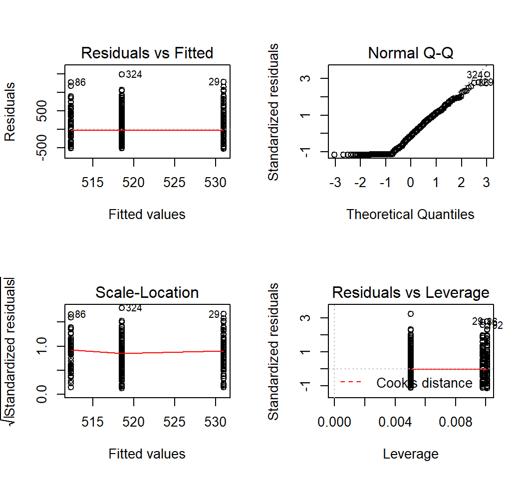
Diagnostics

Diagnostics are the same as those for simple linear regression with a quantitative predictor.

Motivation

• How is sales (in thousands of units) for a particular product related to advertising budgets (in thousands of dollars) for TV, radio and newspaper?

• Model: sales = \(\beta_0\) + \(\beta_1 \times\) TV + \(\beta_2\times\) radio + \(\beta_3 \times\) newspaper + \(\varepsilon\)

We want to examine the relationship between sales and budgets for TV, radio and newspaper jointly, instead of marginally.

Model

Response \(Y\) and \(p\) predictors \(X_1, X_2, \ldots, X_p\), bound by model

\[Y = \beta_0 + \beta_1 X_1 +\beta_2 X_2 + \cdots + \beta_p X_p + \varepsilon\]

• \(\beta_j\): change in units in \(E(Y)\) for a unit change in \(X_j\) while holding all other predictors fixed

• \(\varepsilon\): random error term with \(E(\varepsilon)=0\) and \(Var(\varepsilon)=\sigma^2\)

• Estimate coefficient vector \(\boldsymbol{\beta}=(\beta_0,\beta_1,\ldots,\beta_p)\) by the least squares method; estimate \(\hat{\boldsymbol{\beta}}=(\hat{\beta}_0,\hat{\beta}_1,\ldots,\hat{\beta}_p)\) as LSE (least squares estimate)

Fitting model

Joint model vs marginal model:

# A tibble: 4 x 5
  term        estimate std.error statistic  p.value
  <chr>          <dbl>     <dbl>     <dbl>    <dbl>
1 (Intercept)  2.94      0.312       9.42  1.27e-17
2 TV           0.0458    0.00139    32.8   1.51e-81
3 radio        0.189     0.00861    21.9   1.51e-54
4 newspaper   -0.00104   0.00587    -0.177 8.60e- 1

# A tibble: 2 x 5
  term        estimate std.error statistic  p.value
  <chr>          <dbl>     <dbl>     <dbl>    <dbl>
1 (Intercept)  12.4       0.621      19.9  4.71e-49
2 newspaper     0.0547    0.0166      3.30 1.15e- 3

# A tibble: 2 x 5
  term        estimate std.error statistic  p.value
  <chr>          <dbl>     <dbl>     <dbl>    <dbl>
1 (Intercept)   7.03     0.458        15.4 1.41e-35
2 TV            0.0475   0.00269      17.7 1.47e-42

Testing on all coefficients

• Is there a relationship between the response and any of the predictors? Namely, is \(H_0: \beta_1=\beta_2=\cdots=\beta_p=0\) true?
• Test statistic: F-statistic \[F=\frac{(TSS-RSS)/p}{RSS/(n-p-1)},\] where \(TSS=\sum_{i=1}^n (y_i - \bar{y})^2\) with \(\bar{y}=n^{-1}\sum_{i=1}^n y_i\) and \(RSS=\sum_{i=1}^n (y_i - \hat{y}_i)^2\)
• If \(H_0\) is true and the linear model assumptions are correct, F-statistic should be close to 1 on average; under suitable conditions, F-statistic approximately follows an F-distribution

Testing on all coefficients

Testing \(H_0: \beta_1=\beta_2=\cdots=\beta_p=0\):

   value    numdf    dendf 
570.2707   3.0000 196.0000 
       value 
1.575227e-96 

F-statistic: 570.3 with numerator degrees of freedom 3 and denominator degrees of freedom 196; p-value: < 2.2e-16

• Conclusion: reject \(H_0\), meaning that at least one of the predictors has a relationship with the response.

Testing on some coefficients

Is there no relationship between the response and some predictors? Namely, for some \(1 \le q \le p\), test \[H_0: \beta_{p-q+1}=\beta_{p-q+2}= \ldots = \beta_{p}=0\]

• Fit \(M_0: Y = \beta_0 + \beta_1 X_1 + \ldots + \beta_{p-q} X_{p-q} + \varepsilon\), and obtain its residual sum of squares \(RSS_0\)
• Fit \(M_1: Y = \beta_0 + \beta_1 X_1 + \ldots + \beta_{p-q} X_{p-q} + \ldots + \beta_p X_p+\varepsilon\), and obtain its residual sum of squares \(RSS\)
• Use test statistic \[F = \frac{(RSS_0 - RSS)/q}{RSS/(n-p-1)}\]

Testing on some coefficients

When \(H_0\) and model assumptions are true, test statistic \[F = \frac{(RSS_0 - RSS)/q}{RSS/(n-p-1)}\] approximately follows an F-distribution with numerator degrees of freedom \(q\) and denominator degrees of freedom \(n-p-1\)

Testing on model fit

• \(R^2\) measures the proportion of variance that is explained by the postulated model
• With three predictors:

> FitL3c = lm(sales~TV+radio+newspaper,data=adData)
> summary(FitL3c)$r.squared
[1] 0.8972106

• With one predictor:

> FitL3d = lm(sales~newspaper,data=adData)
> summary(FitL3d)$r.squared
[1] 0.05212045

Interaction terms: I

Consider predicting the average sales (in thousands of dollars) via budgets in advertisement through TV and Radio.

• Model 1: \(E\)(sales) = \(\beta_0\) + \(\beta_1 \times\) TV + \(\beta_2 \times\) Radio

• Model 1: how is the change (in unit) in \(E\)(sales) relates to a unit change in TV and/or Radio?

• Is model 1 sensible when changes (in unit) in \(E\)(sales) are different for a unit change in TV when Radio takes different values?

Interaction terms: I

• If change (in unit) in \(E\)(sales) can be different for a unit change in TV at different values of Radio or for a unit change in Radio at different values of TV, then the model \[ E(\textsf{sales}) = \beta_0 + \beta_1 \times\textsf{TV} + \beta_2 \times\textsf{Radio} \] is no longer suitable
  
• One way to account for this is to introduce an interaction term and use model \[ E(\textsf{sales}) = \beta_0 + \beta_1 \times \textsf{TV} + \beta_2 \times\textsf{Radio} + \beta_3 \times\textsf{TV} \times\textsf{Radio} \]
• Does the following model do the job? \[ E(\textsf{sales}) = \beta_0 + \beta_1 \times \textsf{TV} + \beta_2 \times \textsf{Radio} + \beta_3 \times \textsf{TV}^2+ \beta_4 \times \textsf{Radio}^2 \]

Interaction terms: I

The model \[ E(\textsf{sales}) = \beta_0 + \beta_1 \times \textsf{TV} + \beta_2 \times\textsf{Radio} + \beta_3 \times\textsf{TV} \times\textsf{Radio} \] can be written as \[ E(\textsf{sales}) = \beta_0 + \beta_1 \times \textsf{TV} + (\beta_2+ \beta_3 \times\textsf{TV})\times\textsf{Radio} \] or as \[ E(\textsf{sales}) = \beta_0 + (\beta_1 +\beta_3 \times\textsf{Radio})\times \textsf{TV} + \beta_2 \times\textsf{Radio} \]

Interaction terms: I

Fit the model with interaction:

Call:
lm(formula = sales ~ TV * radio, data = adData)

Residuals:
    Min      1Q  Median      3Q     Max 
-6.3366 -0.4028  0.1831  0.5948  1.5246 

Coefficients:
             Estimate Std. Error t value Pr(>|t|)    
(Intercept) 6.750e+00  2.479e-01  27.233   <2e-16 ***
TV          1.910e-02  1.504e-03  12.699   <2e-16 ***
radio       2.886e-02  8.905e-03   3.241   0.0014 ** 
TV:radio    1.086e-03  5.242e-05  20.727   <2e-16 ***
---
Signif. codes:  0 '***' 0.001 '**' 0.01 '*' 0.05 '.' 0.1 ' ' 1

Residual standard error: 0.9435 on 196 degrees of freedom
Multiple R-squared:  0.9678,    Adjusted R-squared:  0.9673 
F-statistic:  1963 on 3 and 196 DF,  p-value: < 2.2e-16

Interaction terms: II

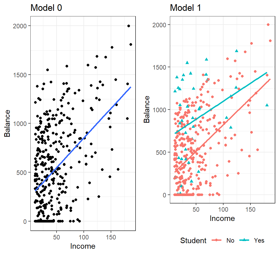
Consider predicting the average Balance (of a credit card) using information on if a user is a Student (“Yes” or “No”) and his/her Income

• Model 0: \(E\)(Balance) = \(\beta_0\) + \(\beta_1 \times\) Income
• Model 1: \(E\)(Balance) = \(\beta_0\) + \(\beta_1 \times\) Student + \(\beta_2 \times\) Income
• Model 2: \(E\)(Balance) = \(\beta_0\) + \(\beta_1 \times\) Student + \(\beta_2 \times\) Income + \(\beta_3 \times\) Student \(\times\) Income

Coding in R: Student=“No” is coded as 0 and the baseline, and Student=“Yes” as 1

Interaction terms: II

Interaction terms: II

Fit the model with interaction:

Call:
lm(formula = Balance ~ Student * Income, data = creditData)

Residuals:
    Min      1Q  Median      3Q     Max 
-773.39 -325.70  -41.13  321.65  814.04 

Coefficients:
                  Estimate Std. Error t value Pr(>|t|)    
(Intercept)       200.6232    33.6984   5.953 5.79e-09 ***
StudentYes        476.6758   104.3512   4.568 6.59e-06 ***
Income              6.2182     0.5921  10.502  < 2e-16 ***
StudentYes:Income  -1.9992     1.7313  -1.155    0.249    
---
Signif. codes:  0 '***' 0.001 '**' 0.01 '*' 0.05 '.' 0.1 ' ' 1

Residual standard error: 391.6 on 396 degrees of freedom
Multiple R-squared:  0.2799,    Adjusted R-squared:  0.2744 
F-statistic:  51.3 on 3 and 396 DF,  p-value: < 2.2e-16

Diagnostics

• Diagnostics for multiple linear regression are very similar to those for simple linear regression with a quantitative predictor.
• Additional task: check on collinearity and variance inflaction factor (VIF)

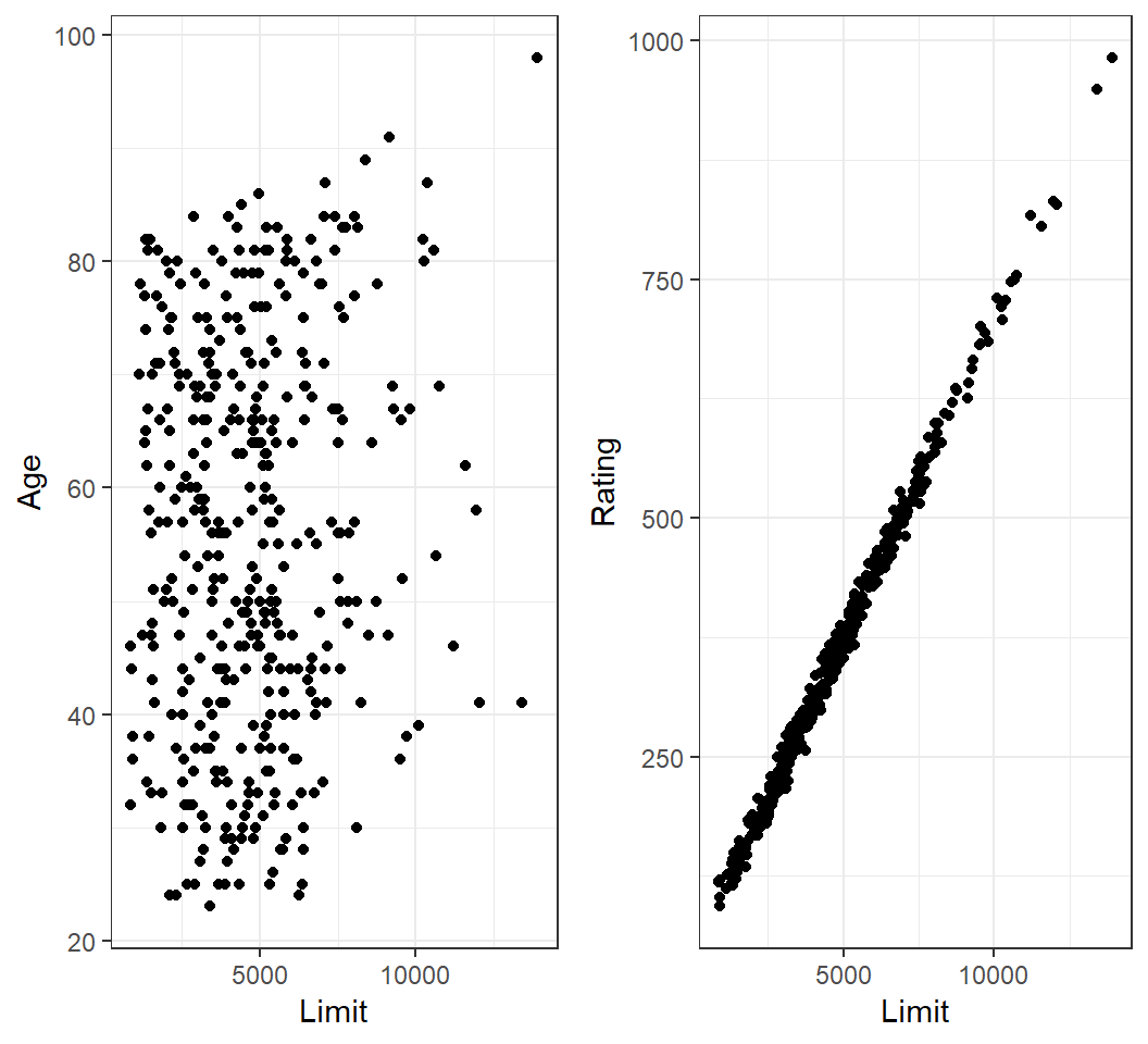
Collinearity

Collinearity

• refers to the situation in which two or more predictor variables are closely related to each other
• often inflates the variances of estimated coefficients and makes the model unstable
• can be measured by the variance inflaction factor (VIF)

A VIF value that exceeds 5 or 10 indicates a problematic amount of collinearity

Note: VIF(\(\hat{\beta}_j) = \frac{1}{1-R^2_{X_j|X_{-j}}}\); collinearity implies \(R^2_{X_j|X_{-j}} \approx 1\)

Collinearity

Collinearity among Limit and Rating:

Colllinearity

Model Balance~Age+Limit:

# A tibble: 3 x 5
  term        estimate std.error statistic   p.value
  <chr>          <dbl>     <dbl>     <dbl>     <dbl>
1 (Intercept) -173.     43.8         -3.96 9.01e-  5
2 Age           -2.29    0.672       -3.41 7.23e-  4
3 Limit          0.173   0.00503     34.5  1.63e-121

Model Balance~Rating+Limit:

# A tibble: 3 x 5
  term         estimate std.error statistic  p.value
  <chr>           <dbl>     <dbl>     <dbl>    <dbl>
1 (Intercept) -378.       45.3       -8.34  1.21e-15
2 Rating         2.20      0.952      2.31  2.13e- 2
3 Limit          0.0245    0.0638     0.384 7.01e- 1

Note: compare standard errors of \(\hat{\beta}_{\textsf{Limit}}\) in both models

Colllinearity

> FitL3f = lm(Balance~Age+Rating+Limit,data=creditData)
> library(car)
> vif(FitL3f)
       Age     Rating      Limit 
  1.011385 160.668301 160.592880 

• VIFs indicate considerable collinearity in the data

In case of collinearity, either drop one of the problematic variables or combine some closely related variables

Non-linear relationship

If there is evidence on a non-linear relationship between response and predictors, we can

• add high-order terms into the model (or employ more advanced non-linear methods); e.g., \[E(Y)=\beta_0+\beta_1 X + \beta_2 X^2\]
• transform predictors (and/or response); e.g., e.g., \(E(Y)=\beta_0+\beta_1 \times f(X)\), where \(f\) can be \(\log(X)\) or \(\sqrt{X}\)

License and session Information

License

> sessionInfo()
R version 3.5.0 (2018-04-23)
Platform: x86_64-w64-mingw32/x64 (64-bit)
Running under: Windows 10 x64 (build 19041)

Matrix products: default

locale:
[1] LC_COLLATE=English_United States.1252 
[2] LC_CTYPE=English_United States.1252   
[3] LC_MONETARY=English_United States.1252
[4] LC_NUMERIC=C                          
[5] LC_TIME=English_United States.1252    

attached base packages:
[1] stats     graphics  grDevices utils     datasets  methods  
[7] base     

other attached packages:
[1] car_3.0-2     carData_3.0-2 broom_0.5.1   gridExtra_2.3
[5] ggplot2_3.1.0 knitr_1.21   

loaded via a namespace (and not attached):
 [1] revealjs_0.9      tidyselect_0.2.5  xfun_0.4         
 [4] purrr_0.2.5       haven_2.0.0       lattice_0.20-35  
 [7] colorspace_1.3-2  generics_0.0.2    htmltools_0.3.6  
[10] yaml_2.2.0        utf8_1.1.4        rlang_0.4.4      
[13] pillar_1.3.1      foreign_0.8-70    glue_1.3.0       
[16] withr_2.1.2       readxl_1.2.0      plyr_1.8.4       
[19] stringr_1.3.1     cellranger_1.1.0  munsell_0.5.0    
[22] gtable_0.2.0      zip_1.0.0         evaluate_0.12    
[25] labeling_0.3      rio_0.5.16        forcats_0.3.0    
[28] curl_3.2          fansi_0.4.0       Rcpp_1.0.3       
[31] scales_1.0.0      backports_1.1.3   abind_1.4-5      
[34] hms_0.4.2         digest_0.6.18     openxlsx_4.1.0   
[37] stringi_1.2.4     dplyr_0.8.4       grid_3.5.0       
[40] cli_1.0.1         tools_3.5.0       magrittr_1.5     
[43] lazyeval_0.2.1    tibble_2.1.3      crayon_1.3.4     
[46] tidyr_0.8.2       pkgconfig_2.0.2   data.table_1.11.8
[49] assertthat_0.2.0  rmarkdown_1.11    rstudioapi_0.8   
[52] R6_2.3.0          nlme_3.1-137      compiler_3.5.0