Stat 435 Lecture Notes 5b
Xiongzhi Chen
Washington State University
Different Error Measures
Hypothesis testing
- Null hypothesis \(H_0\): natural status
Alternative hypothesis \(H_1\): status under intervention; complement to \(H_0\)
Test statistic \(T\), rejection region \(\mathcal{T}\) and rejection rule \(\mathcal{R}\): reject \(H_0\) if \(T \in \mathcal{T}\)
- Type I error \(\alpha\): probability of rejecting \(H_0\) when it is true
- Type II error \(\gamma\): probability of not rejecting \(H_0\) when \(H_0\) is false
Power: \(1- \gamma\)
Example 1: One Hypothesis
Linear model: \(E(Y) = \beta_0 + \beta_1 X\)
\(H_0: \beta_1 =0\) versus \(H_1:\beta_1 \ne 0\)
Pick type I error level \(\alpha \in (0,1)\)
Test statistic \(T\); reject \(H_0\) if \(\vert T \vert > c_{\alpha}\)
How to interpret \(\alpha\)?
Example 2: Many Hypotheses
Linear model: \(E(Y) = \beta_0 + \beta_1 X + \cdots + \beta_{m} X_{m}\)
\(H_{i0}: \beta_i =0\) versus \(H_{i1}:\beta_i \ne 0\), \(i=1,\ldots,m\)
Test all \(H_{i0},i=1,\ldots,m\) simultaneously
If each \(H_{i0}, i=1,\ldots,m\) is tested individually at type I error level \(\alpha\), what will happen to the number of rejected true null hypotheses?
Family-wise error rate (FWER)
\(H_{i0}: \beta_i =0\) versus \(H_{i1}:\beta_i \ne 0\), \(i=1,\ldots,m\)
Rejection of a true null hypothesis is called “false rejection’’
\(V\): number of false rejections, i.e., rejected true \(H_{i0}\)’s
Family-wise error rate (FWER): \[\Pr(V \ge 1) = 1 - \Pr(V=0)\]
Control FWER: \(\Pr(V \ge 1) \le \alpha\)
Family-wise error rate (FWER)
Widely used, e.g., by FDA
Good when there are only a few hypotheses to test simultaneously
Too stringent when there are many hypotheses to test simultaneously, and hence may suffer loss in power
What about controlling “k-FWER”, i.e., \[\Pr(V \ge k) \le \alpha ?\]
False Discovery Rate
False discovery rate
Allow false rejections, and hence much less stringent than FWER
Modern standard on testing many hypotheses simultaneously
- Scalable to many, many hypotheses simultaneously
- GWAS study with a few millions of hypotheses to test simultaneously
- Gene expression study with a few thousand hypotheses to test simultaneously
A standard criterion in model/variable selection
Classification table
- \(H_{i0}: \beta_i =0\) versus \(H_{i1}:\beta_i \ne 0\), \(i=1,\ldots,m\)
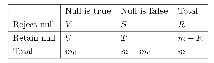
False discovery rate (FDR)
\(\mathcal{R}\): decision rule
\(V\): number of false rejections
\(R\): number of rejections
False discovery proportion: \(\mathrm{FDP}(\mathcal{R}) = V/\max\{R,1\}\)
False discovery rate: \[\mathrm{FDR}(\mathcal{R}) = E\left[\frac{V}{\max\{R,1\}}\right]\]
FDR: Example
\(m=5\) hypothesis \(H_{i0}: \beta_i =0, i=1,2,3,4,5\)
\(H_{i0},i=1,2,3\) are true nulls
Decision rule \(\mathcal{R}\) rejects \(H_{i1}, H_{i2},H_{i4}, H_{i5}\)
What is the false discovery proportion?
Control false discovery rate
Computing exact false discovery rate can be quite difficult
- Control FDR at a nominal level:
Pick a nominal level \(\alpha \in (0,1)\)
Find a decision rule \(\mathcal{R}\), such that \[ \mathrm{FDR}(\mathcal{R}) \le \alpha \]
Find such a decision rule can be hard in general
Benjamini-Hochberg procedure
Benjamini-Hochberg procedure
- Given: \(m\) null hypotheses \(H_{i0}\)
- Given: \(m\) p-values; \(p_i\) for testing \(H_{i0}\)
- Benjamini-Hochberg (BH) procedure
- Order p-values into \(p_{(1)} \le p_{(2)} \le \cdots \le p_{(m)}\)
- Set \(r = \max \left\{ k \in \{1,\ldots,m \}: p_{(i)} \le i \alpha m^{-1} \right\}\)
- Rejection rule:
- If \(r\) is defined, reject the \(r\) \(H_{i0}\)’s corresponding to \(p_{(1)},\ldots,p_{(r)}\)
- If \(r\) is not defined, do not reject any \(H_{i0}\)
- Under some conditions, FDR of BH procedure is upper bounded by \(\alpha\)
BH procedure: example
\(5\) hypotheses \(H_{10}, H_{20},H_{30},H_{40},H_{50}\)
\(p_1 = 0.03\), \(p_2 = 0.1\), \(p_3 = 0.02\), \(p_4 = 0.05\), \(p_5 = 0.02\)
Implement BH procedure at nominal FDR level \(\alpha =0.05\)
Post-selection inference
Linear model and LASSO
Model: \[Y=\beta_0+\beta_1 X_1 + \beta_2 X_2 + \ldots + \beta_p X_p + \varepsilon\]
The LASSO estimate \(\hat{\boldsymbol{\beta}}^L_{\lambda}=(\hat{\beta}_1,\ldots,\hat{\beta}_p)\) is the \({\boldsymbol{\beta}}=({\beta}_1,\ldots,{\beta}_p)\) that minimizes \[ L_1(\beta_0,\boldsymbol{\beta},\lambda)= \frac{1}{2}\sum_{i=1}^n (y_i - \hat{y}_i)^2 + \lambda \sum_{i=1}^p\vert \beta_i \vert \]
The optimal value \(\lambda^{\ast}\) of the tuning parameter \(\lambda\) is often determined by \(k\)-fold cross-validation
Linear Ridge regression
Model: \[Y=\beta_0+\beta_1 X_1 + \beta_2 X_2 + \ldots + \beta_p X_p + \varepsilon\]
The LASSO estimate \(\hat{\boldsymbol{\beta}}^R_{\lambda}=(\hat{\beta}_1,\ldots,\hat{\beta}_p)\) is the \({\boldsymbol{\beta}}=({\beta}_1,\ldots,{\beta}_p)\) that minimizes \[ L_1(\beta_0,\boldsymbol{\beta},\lambda)= \frac{1}{2}\sum_{i=1}^n (y_i - \hat{y}_i)^2 + \lambda \sum_{i=1}^p \beta_i^2 \]
The optimal value \(\lambda^{\ast}\) of the tuning parameter \(\lambda\) is often determined by \(k\)-fold cross-validation
Penalized logistic regression
- LASSO logistic regression when some \(\beta_{i}\)’s are zero: \[ \hat{\beta}=\left( \hat{\beta}_{0},\hat{\beta}_{1},\ldots,\hat{\beta} _{m}\right) \in\operatorname*{argmin}_{\beta}\left[ -\log L\left( \beta\right) +\lambda\sum_{j=1}^{m}\left\vert \beta_{j}\right\vert \right] \]
- Ridge logistic regression: \[ \hat{\beta}=\left( \hat{\beta}_{0},\hat{\beta}_{1},\ldots,\hat{\beta} _{m}\right) \in\operatorname*{argmin}_{\beta}\left[ - \log L\left( \beta\right) +\lambda\sum_{j=1}^{m}\left\vert \beta_{j}\right\vert ^{2}\right] \]
- The optimal value \(\lambda^{\ast}\) of the tuning parameter \(\lambda\) is often determined by \(k\)-fold cross-validation
Note: \(\operatorname*{argmin}_{\beta}\) refers to optimal \(\beta^{\ast}\) which minimizes the corresponding objective function
Post-selection inference
Post-selection inference often aims at controlling false discovery rate (FDR)
Benjamini-Hochberg procedure is used to control FDR
Bias correction method or knock-off method can be used
Note: Please see practice files
License and session Information
> sessionInfo()
R version 3.5.0 (2018-04-23)
Platform: x86_64-w64-mingw32/x64 (64-bit)
Running under: Windows 10 x64 (build 19045)

Matrix products: default

locale:
[1] LC_COLLATE=English_United States.1252
[2] LC_CTYPE=English_United States.1252
[3] LC_MONETARY=English_United States.1252
[4] LC_NUMERIC=C
[5] LC_TIME=English_United States.1252

attached base packages:
[1] stats     graphics  grDevices utils     datasets  methods
[7] base

other attached packages:
[1] knitr_1.21

loaded via a namespace (and not attached):
 [1] compiler_3.5.0  magrittr_1.5    tools_3.5.0
 [4] htmltools_0.3.6 revealjs_0.9    yaml_2.2.0
 [7] Rcpp_1.0.12     stringi_1.2.4   rmarkdown_1.11
[10] stringr_1.3.1   xfun_0.4        digest_0.6.18
[13] evaluate_0.13