Overview

• Linear models are simple (e.g., easy to fit and interpret) but quite inflexible, since often linearity assumption is a poor approximation

• We need to look beyond linear models, and choose models that somehow are not too complicated but flexible enough to considerably improve upon linear models

• We will discuss four types of models: polynomial regression, spline models, and generalized additive models

Model

Scalar predictor \(X\) and scalar response \(Y\):

• Population version: \[Y=\beta_{0}+\beta_{1}X+\beta_{2}X^{2}+\cdots+\beta_{d}X^{d}+\varepsilon, \mathbb{E}(\varepsilon)=0\]
• Data version: \[y_{i}=\beta_{0}+\beta_{1}x_{i}+\beta_{2}x_{i}^{2}+\cdots+\beta_{d}x_{i}% ^{d}+\varepsilon_{i}, \mathbb{E}(\varepsilon_i)=0\]
• \(\beta_{0},...,\beta_{d}\) can be estimated by the least squares method, by pretending that \(x_{i}^{j}\) for each \(j\in\left\{ 1,...,d\right\}\) is a predictor when the associated design matrix does not behave badly

Boundary effect

• Usually \(d=3\) or \(4\) is set since the polynomial \[ f\left( x\right) =\beta_{0}+\beta_{1}x+\beta_{2}x^{2}+\cdots+\beta_{d}x^{d} \] may behave wildly

• Reason: dominant term \(\beta_{d}X^{d}\) (when \(\beta_{d}\neq0\)) varies wildly near boundary of observed \(X\) variable

• Caution: Boundary effect is a common problem for complicated models, and there are strategies to mitigate this

Estimated model

• Estimate of \(f\): \[ \hat{f}\left( x\right) =\hat{\beta}_{0}+\hat{\beta}_{1}x+\hat{\beta}% _{2}x^{2}+\cdots+\hat{\beta}_{d}x^{d} \]

• Covariance matrix of \(\hat{\beta}=\left( \hat{\beta}_{0} ,\hat{\beta}_{1},\hat{\beta}_{2},...,\hat{\beta}_{d}\right) ^{T}\) as \(\mathbf{C}\)

• \(\mathbf{C}\) can be complicated

Confidence band

• Variance of \(\hat{f}\left(x\right)\) for a fixed \(x\) is \[\begin{align*} Var\left[ \hat{f}\left( x\right) \right] & =\underbrace{\left( 1,x,x^{2},...,x^{d}\right) }_{l_{d}^{T}\left( x\right) }\mathbf{C}% \underbrace{\left( 1,x,x^{2},...,x^{d}\right) ^{T}}_{l_{d}\left( x\right) }\\ & =l_{d}^{T}\left( x\right) \mathbf{C}l_{d}\left( x\right) \end{align*}\]
• Envelope for \(\hat{f}\left( x\right)\) formed by: \[ \hat{f}\left( x\right) \pm 2\sqrt{Var\left[ \hat{f}\left( x\right) \right] } \]

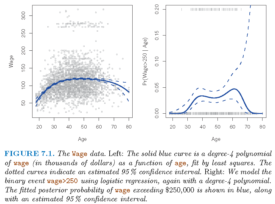
Illustration: model

• Model family: \[ \Pr\left( y_{i}>250|x_{i}\right) =\frac{\exp\left( \theta_{i}\right) }{1+\exp\left( \theta_{i}\right) } \] with \[ \theta_{i}=\beta_{0}+\beta_{1}x_{i}+\beta_{2}x_{i}^{2}+\cdots+\beta_{d}% x_{i}^{d} \]
• \(d=1\) gives simple logistic regression

Illustration: fitted

Basis functions

• \(\left(d+1\right)\) monomials \(1,X,X^{2},...,X^{d}\) generate polynomials \(\mathcal{P}_d\) of degree \(d\) with elements: \[ f_d(x)=\beta_{0}+\beta_{1}x+\beta_{2}x^{2}+\cdots+\beta_{d}x^{d} \]

• \(d\) functionally linearly independent functions \(f_{1},...,f_{d}\) generate family \(\mathcal{F}\) with elements \[\begin{equation} \tilde{f}\left( x\right) =\beta_{0}+\beta_{1}f_{1}\left( x\right) +\beta_{2}f_{2}\left( x\right) +\cdots+\beta_{d}f_{d}\left( x\right) \end{equation}\]

• \(\left\{ f_{i}\right\} _{i=1}^{d}\) are called basis functions for \(\mathcal{F}\)

• Note: these are concepts in linear algebra

Piecewise polynomials

• A global polynomial regression model has intrinsic disadvantages

• Alternative strategy: fit different polynomial regressions on different parts of data, by requiring these polynomials to be consistent in some sense, so that the resultant model displays some stability as it transits from one part of data to the other

• Consider the model \(M\): \[ Y=\left\{ \begin{array} [c]{cc}% \beta_{01}+\beta_{11}X+\beta_{21}X^{2}+\beta_{31}X^{3}, & X<c\\ \beta_{02}+\beta_{12}X+\beta_{22}X^{2}+\beta_{32}X^{3}, & X\geq c \end{array} \right. \]

Piecewise polynomials

• Data version \[ y_{i}=\left\{ \begin{array} [c]{cc}% \beta_{01}+\beta_{11}x_{i}+\beta_{21}x_{i}^{2}+\beta_{31}x_{i}^{3}, & x_{i}<c\\ \beta_{02}+\beta_{12}x_{i}+\beta_{22}x_{i}^{2}+\beta_{32}x_{i}^{3}, & x_{i}\geq c \end{array} \right. \]

• \(M\) has two sub-models, \(M_{1}\) and \(M_{2}\), on two distinct parts, \(D_{1}=\left\{ \left( X,Y\right) :X<c\right\}\) and \(D_{2}=\left\{ \left( X,Y\right) :X\geq c\right\}\), of data space

• \(c\) for \(X\) is where \(M\) transits from \(M_{1}\) to \(M_{2}\) (or vice versa); \(c\) is called a “knot”

Splines

• Splines are a type of regression polynomials:
  • They employ polynomials up to a fixed degree
  • Where two polynomials meet, some constrains are satisfied
• Cubic splines employ \(\deg(3)\) polynomials
• Natural splines also satisfy linear constraints at boundary
• Smoothing splines directly satisfy smoothness constraints and need not to have polynomial components

Cubic splines

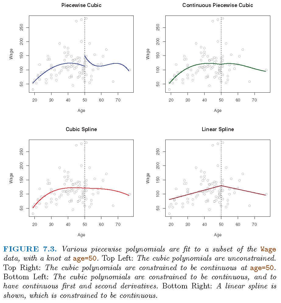
• Two cases of transition of \(M\) from \(M_{1}\) to \(M_{2}\):

  • Case 1: \(M_{1}\) does not match \(M_{2}\) at \(c\); e.g., \(M\) jumps from \(M_{1}\) to \(M_{2}\) at \(c\)
  • Case 2: \(M_{1}\) matches \(M_{2}\) at \(c\) in some sense; e.g., \(M_{1}\) matches \(M_{2}\) at \(c\), in value, (and/or) in speed of change, (and/or) in curvature

• For practical purposes it is often desirable to have Case 2, and the \(3\)-degree polynomials with matching values (i.e., \(M\) itself is continuous), speeds (i.e., first-order derivatives) and curvatures (i.e., second-order derivatives) at each knot are called cubic splines

Illustration

Smoothing splines

• Split the range of \(X\) into \(K+1\) parts and only employ polynomials of degree \(d\); so needing \(K\) knots and \(K+1\) such polynomials

• Restrict these polynomials such that there are \(s\) constrains for each distinct pair of them at a knot, then we have \(p=T-C\) parameters to estimate

• \(T = (K+1) \times (d+1)\); \((K+1)\) number of distinct regions of values of \(X\), and \(d+1\) number of parameters in each polynomial

• \(C = K \times s\); \(K\) number of knots and \(s\) number of constraints at each knot

Smoothing splines

In the above formula, \(s\), the number of constraints at each knot can be understood as follows:

• If submodels \(M_{i}\) and \(M_{i+1},i=1,...,K\) match in their values and up to their \(\left( s-1\right)\)-th order derivatives at each knot \(Q_{i}\), then at knot \(Q_{i}\) there are \(s\) constraints on their associated polynomials

• If we take \(0\)-th order derivative as performing no differentiation but keeping original function untouched, then \(M_{i}\) and \(M_{i+1},i=1,...,K\) matching up to their \(r\)-th order derivatives at each knot \(Q_{i}\) induces \(r+1\) constraints

Smoothing splines: representation

• Consider \(d=3\). A cubic spline with \(K\) knots can be modelled as \[ y_{i}=\beta_{0}+\beta_{1}b_{1}\left( x_{i}\right) +...+\beta_{K+3}b_{K+3}\left( x_{i}\right) +\varepsilon_{i} \] for an appropriate choice of basis functions \(b_{1},b_{2},...,b_{K+3}\)

• One such basis is partially induced by the function \[ h\left( x,\xi\right) =\left( x-\xi\right) _{+}^{3}=\left\{ \begin{array} [c]{cc}% \left( x-\xi\right) ^{3}, & x>\xi\\ 0, & x\leq\xi \end{array} \right. \]

Smoothing splines: representation

• In summary, to fit a cubic spline to a data set with \(K\) knots, we can equivalently fit the model \[ Y=\beta_{0}+\beta_{1}X+\beta_{2}X^{2}+\beta_{3}X^{3}+\\ \beta_{4}% \underbrace{h\left( X,\xi_{1}\right) }_{\text{the 4th predictor}}% +...+\beta_{K+3}h\left( X,\xi_{K}\right) +\varepsilon \] or its data version \[ y_{i}=\beta_{0}+\beta_{1}x_{i}+\beta_{2}x_{i}^{2}+\beta_{3}x_{i}^{3}+\\ \beta_{4}h\left( x_{i},\xi_{1}\right) +...+\beta_{K+3}h\left( x_{i},\xi _{K}\right) +\varepsilon_{i} \] where \(\xi_{1},...,\xi_{K}\) are the knots
• Fitting this model uses \(K+4\) degrees of freedom. We can use the least squares method to fit the model

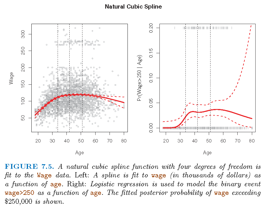
Natural splines

• As for any regression that employs a polynomial, fitted model may be unstable near or at the boundary (induced by observed values of predictors)

• A natural spline is a regression spline which is required to be linear at the boundary (in the region where \(X\) is smaller than the smallest knot, or larger than the largest knot)

Natural/Cubic spline

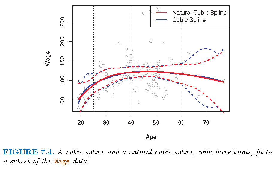
• Each cubic spline has 3 knots

More knots?!

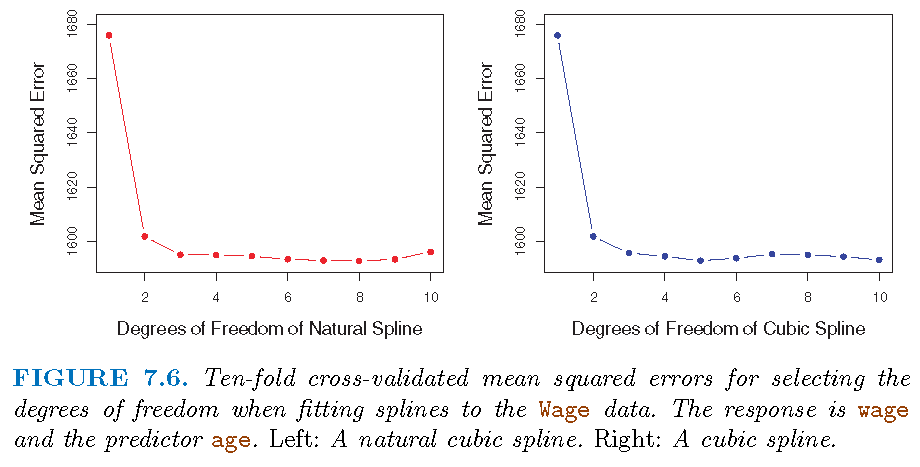
• Regression spline is most flexible in regions that contain a lot of knots, because in those regions the polynomial coefficients can change rapidly. Hence, one option is to place more knots in places where we feel the function might vary most rapidly, and to place fewer knots where it seems more stable

• While this option can work well, in practice it is common to place knots in a uniform fashion. One way to do this is to specify the desired degrees of freedom, and then have the software automatically place the corresponding number of knots at uniform quantiles of the data, as done, e.g., by \(10\)-fold CV based on the residual sum of squares (RSS) values

Placing knots

• \(3\) knots, placed at 25th, 50th, 75th percentiles of age

Choosing knots

Comparison

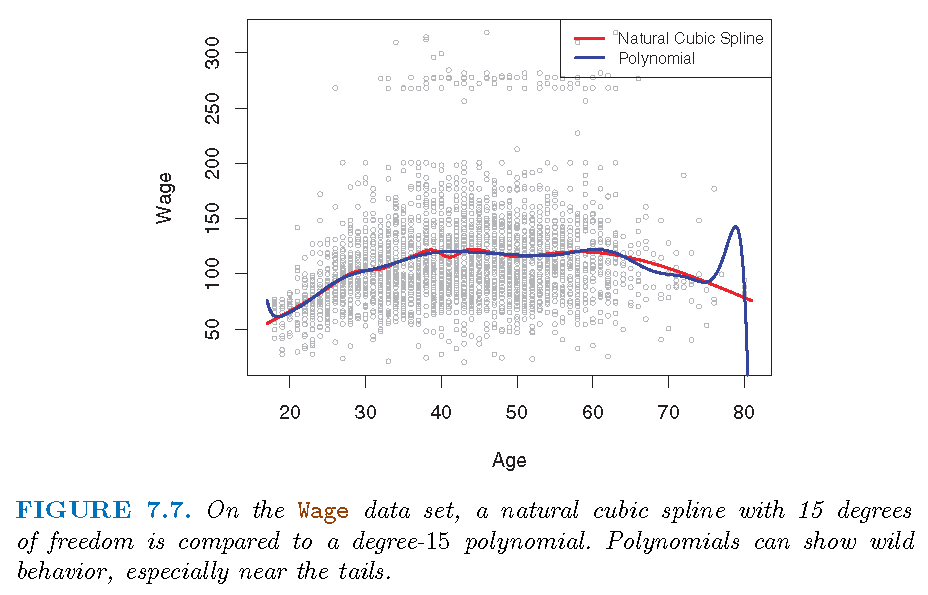
“Regression splines often give superior results to polynomial regression”:

• To be more flexible, polynomial regressions resort to higher degree polynomials which results in added instability at boundary (of observations for \(X\)).

• Splines only need to plan for better knots in order to achieve flexibility, and natural splines alleviate instability at boundary

• Spline captures much better (than polynomial regression) local behavior of \(f\) in true model \(E(Y|X)=f(X)\) where \(f\) changes rapidly.

Illustration

Motivation

Smoothing splines are splines produced directly by restricting how smooth a candidate function can be:

• Given the data \(\left\{ \left( x_{i},y_{i}\right) :i=1,...n\right\}\), there is a function \(g\) such that \(\sum_{i=1}^{n}\left( y_{i}-g\left( x_{i}\right) \right)^{2}=0\)

• In terms of the local properties of \(g\) such as continuity and differentiability, we can restrict the integrated curvature of \(g\), which is \(\int\left[ g^{\prime\prime}\left( t\right) \right] ^{2}dt\). The integral essentially restricts how variable \(g^{\prime\prime}\) is (and hence approximately how variable the curvature of \(g\) is)

Formulation

• A function \(g\) that minimizes \[\begin{equation} \underbrace{\sum_{i=1}^{n}\left( y_{i}-g\left( x_{i}\right) \right) ^{2} }_{\text{squared loss}}+\underbrace{\lambda\int\left[ g^{\prime\prime}\left( t\right) \right] ^{2}dt}_{\text{penalty on smoothness}} \label{eq76}% \end{equation}\]

  (for each fixed \(\lambda\geq0\)) is called a smoothing spline

• When is \(g^{\prime\prime}\left( t\right)\) a constant?
• For practical usage, \(\deg\left( g\right) \ge 3\) if \(g\) is a polynomial

• Penalty term referred to as roughness penalty

Key observations

• When \(\lambda=0\), the penalty term has no effect and \(g\) can be discontinuous and will exactly interpolate the data

• When \(\lambda\neq0\), \(g\) has to be twice differentiable in order to possess a second order derivative

• When \(\lambda=\infty\), the minimizer \(\hat{g}\) must satisfy \(\hat{g}^{\prime\prime}\left( t\right) =0\). This means that \(\hat {g}\) has to be a linear function, i.e., \(\hat{g}\left( x\right) =\beta _{0}+\beta_{0}x\), in which case we get linear regression

Complexity and performance

The minimizer \(\hat{g}_{\lambda}\) for \(\lambda\in\left( 0,1\right)\), being a shunken version of a natural cubic spline, has the following properties:

• \(\hat{g}_{\lambda}\) is a piecewise cubic polynomial with knots at the unique values of \(x_{1},...,x_{n}\)

• \(\hat{g}_{\lambda}\) has continuous first and second order derivatives at each knot

• \(\hat{g}_{\lambda}\) is linear in the region outside of the extreme knots

Proof of the above is a bit complicated and uses machinery from functional analysis and differential equations

Degrees of freedom

• Tuning parameter \(\lambda\) controls the effective degrees of freedom, \(df_{\lambda}\), of \(\hat{g}\)

• \(df_{\lambda}\) decreases from \(n\) to \(2\) as \(\lambda\) increases from \(0\) to \(\infty\)

• \(df_{\lambda}\) measures flexibility of \(\hat {g}_{\lambda}\), in the sense that larger \(df_{\lambda}\) induces a more flexible \(\hat{g}_{\lambda}\)

Degrees of freedom

• Let \(\mathbf{S}_{\lambda}\in\mathbb{R}^{n\times n}\) be formed by evaluating associated basis functions at the \(x_{i}\)’s. Then \[ \mathbf{\hat{g}}_{\lambda}=\left( \begin{array} [c]{c}% \hat{g}_{\lambda}\left( x_{1}\right) \\ \hat{g}_{\lambda}\left( x_{2}\right) \\ \vdots\\ \hat{g}_{\lambda}\left( x_{n}\right) \end{array} \right) =\mathbf{S}_{\lambda}\left( \begin{array} [c]{c}% y_{1}\\ y_{2}\\ \vdots\\ y_{n}% \end{array} \right) \]

• Effective degrees of freedom is defined as \[ df_{\lambda}=\sum_{i=1}^{n}\mathbf{S}_{\lambda}\left( i,i\right) , \] where \(\mathbf{S}_{\lambda}\left( i,j\right)\) is the \(\left( i,j\right)\) entry of \(\mathbf{S}_{\lambda}\)

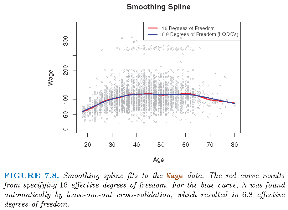
Choose tuning parameter

• Best \(\lambda\) achieves the smallest cross-validation RSS among a grid values of \(\lambda\)

• Quick computation via Leave-one-out-cross-validation (LOOCV) in a single pass on the whole data: \[ RSS_{cv}\left( \lambda\right) =\sum_{i=1}^{n}\left( y_{i}-\hat{g}_{\lambda }^{\left( -i\right) }\left( x_{i}\right) \right) ^{2}\\=\sum_{i=1} ^{n}\left[ \frac{y_{i}-\hat{g}_{\lambda}\left( x_{i}\right) } {1-\mathbf{S}_{\lambda}\left( i,i\right) }\right] ^{2} \]
  • \(\hat{g}_{\lambda}^{\left( -i\right) }\): fitted on \(\left\{ \left( x_{j},y_{j}\right) :j\neq i\right\}\)
  • \(\hat{g}_{\lambda}\): fitted on \(\left\{ \left( x_{i},y_{i}\right) :i=1,...,n\right\}\)

Illustration

Overview

• Generalized additive models (GAMs) employs a non-linear function for each predictor while maintaining additivity of the transformed predictors

• GAMs can be applied to both quantitative and qualitative responses

• Consider \[ y_{i}=\beta_{0}+\beta_{1}x_{i1}+\beta_{2}x_{i2}+\cdots+\beta_{p}% x_{ip}+\varepsilon_{i} \]

• Replace \(\beta_{j}x_{ij}\) by \(f_{j}\left( x_{ij}\right)\) to get a GAM as \[ y_{i}=\beta_{0}+f_{1}\left( x_{i1}\right) +f_{2}\left( x_{i2}\right) +\cdots+f_{p}\left( x_{ip}\right) +\varepsilon_{i} \] for a set of known functions \(\left\{ f_{j}\right\} _{j=1}^{p}\)

Illustration: I

• \(f_{1}\) and \(f_{2}\) natural splines; \(f_{3}\) piecewise constant: \[ \text{wage }=\text{ }\beta_{0}+f_{1}\left( \text{year}\right) +f_{2}\left( \text{age}\right) +f_{3}\left( \text{education}\right) +\varepsilon \]

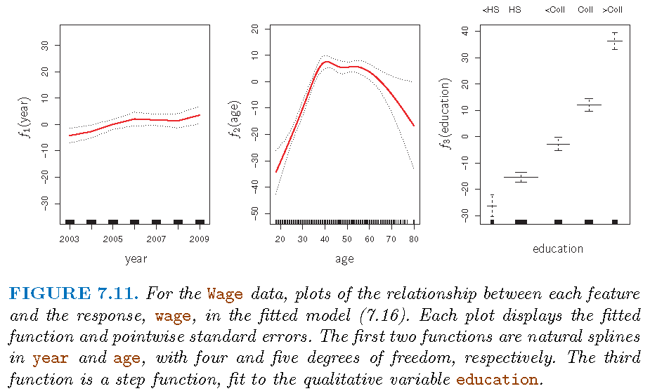
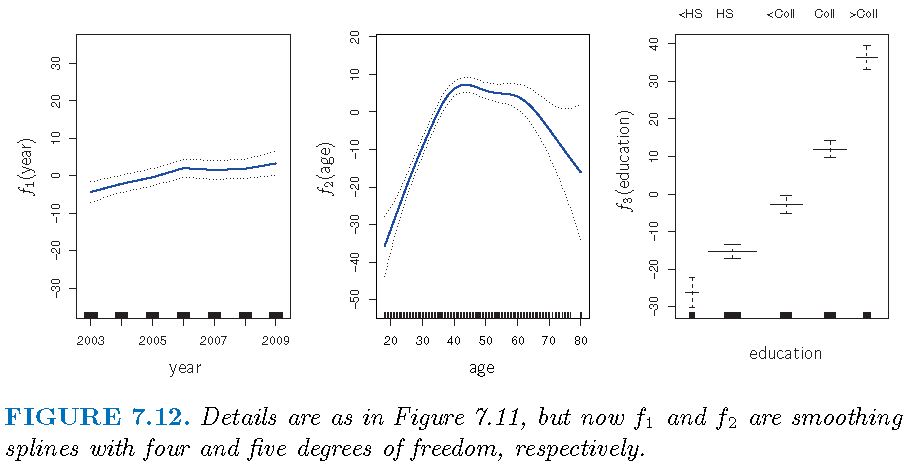
Illustration: II

GAM logistic Reg

• A binary response, linear version: \[ \log\left( \frac{\Pr\left( Y=1|X\right) }{1-\Pr\left( Y=1|X\right) }\right) \\ =\beta_{0}+\beta_{1}x_{i1}+\beta_{2}x_{i2}+\cdots+\beta_{p}% x_{ip}+\varepsilon_{i}% \]

• GAM version: \[ \log\left( \frac{\Pr\left( Y=1|X\right) }{1-\Pr\left( Y=1|X\right) }\right) \\=\beta_{0}+f_{1}\left( x_{i1}\right) +f_{2}\left( x_{i2}\right) +\cdots+f_{p}\left( x_{ip}\right) +\varepsilon_{i}% \]

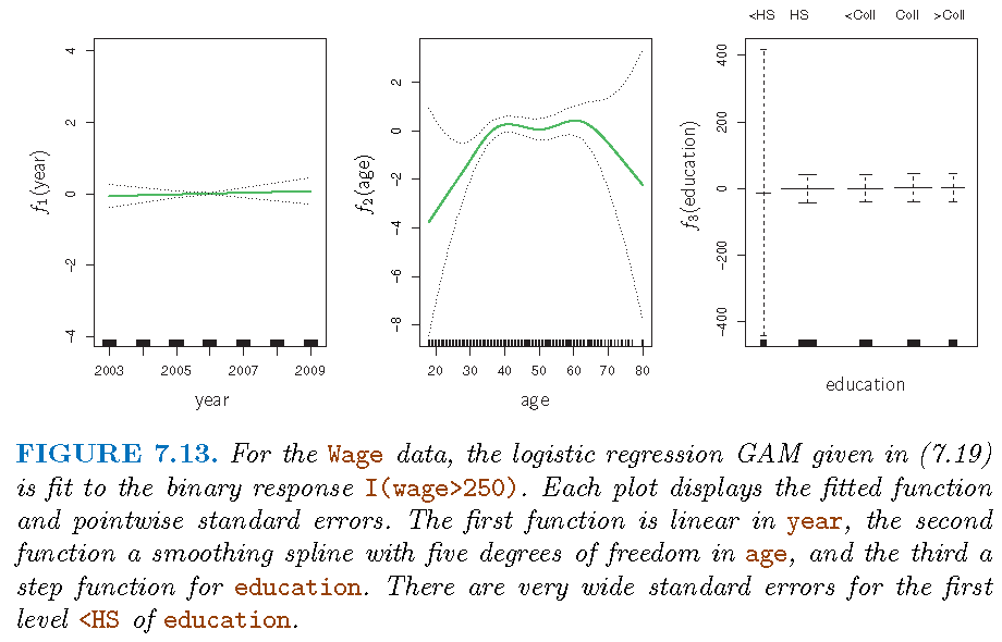
Illustration: III

• Predict \[p\left( X\right) =\Pr\left( \text{wage} >250|\text{year,age,education}\right)\]

• Model: \[ \log\left( \frac{p\left( X\right) }{1-p\left( X\right) }\right) \\ =\beta_{0}+\beta_{1}\times\text{year}+f_{2}\left( \text{age}\right) +f_{3}\left( \text{education}\right) \]

• Note: there are no individuals with less than a high school education who earn over $250,000 per year

Illustration: III

• GAMs are implemented by R library gam

License and session Information

License

> sessionInfo()
R version 3.5.0 (2018-04-23)
Platform: x86_64-w64-mingw32/x64 (64-bit)
Running under: Windows 10 x64 (build 19044)

Matrix products: default

locale:
[1] LC_COLLATE=English_United States.1252 
[2] LC_CTYPE=English_United States.1252   
[3] LC_MONETARY=English_United States.1252
[4] LC_NUMERIC=C                          
[5] LC_TIME=English_United States.1252    

attached base packages:
[1] stats     graphics  grDevices utils     datasets  methods  
[7] base     

other attached packages:
[1] knitr_1.21

loaded via a namespace (and not attached):
 [1] compiler_3.5.0  magrittr_1.5    tools_3.5.0    
 [4] htmltools_0.3.6 revealjs_0.9    yaml_2.2.0     
 [7] Rcpp_1.0.12     stringi_1.2.4   rmarkdown_1.11 
[10] stringr_1.3.1   xfun_0.4        digest_0.6.18  
[13] evaluate_0.13