Overview
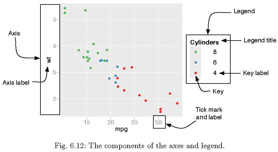
Legend
Brief syntax:
theme(
# Legend position: right, left, bottom, top, none
legend.position = "right",

# Legend background
legend.background = element_rect(fill, color, size, linetype),

# Legend direction and justification, i.e.,
# layout of items in legends ("horizontal" or "vertical")
legend.direction = NULL,

# Legend box, i.e.,
# arrangement of multiple legends ("horizontal" or "vertical")
legend.box = NULL
)
Illustration
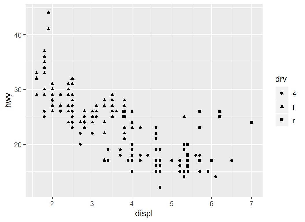
Plot displ vs hwy with shape=drv:
> library(ggplot2)
> p = ggplot(mpg,aes(displ,hwy,shape=drv)) + geom_point()
- due to
shape=drv, a legend with title drv will be created
- by default, the legend title is the variable name
drv
- by default, the legend appears to the right side of the plot, and is centered vertically
Illustration: base layer
> p
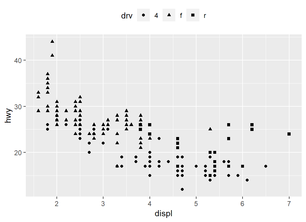
Legend: top, horizontal
> p+theme(legend.position = "top",
+         legend.direction = "horizontal")
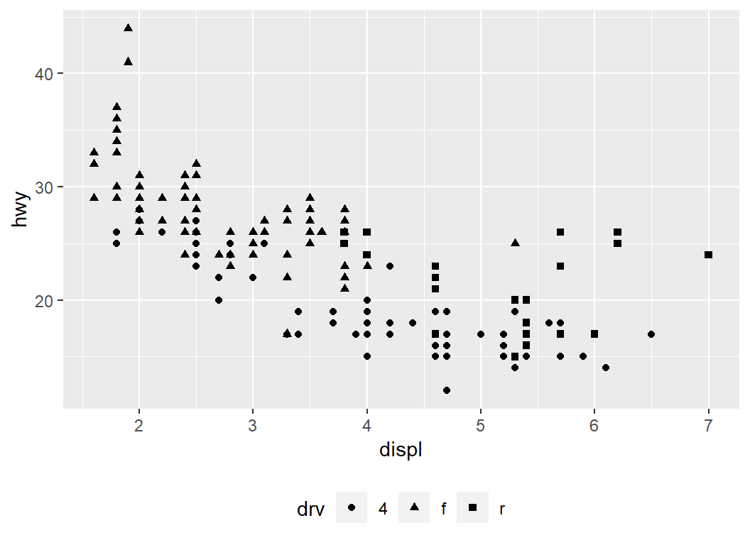
Legend: bottom, horizontal
> p+theme(legend.position = "bottom",
+      legend.direction = "horizontal")
Legend: bottom, vertical
> p+theme(legend.position = "bottom",
+     legend.direction = "vertical")
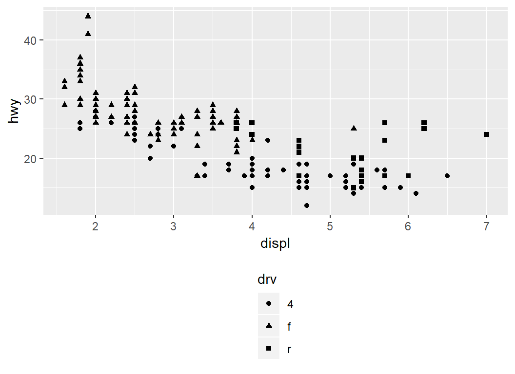
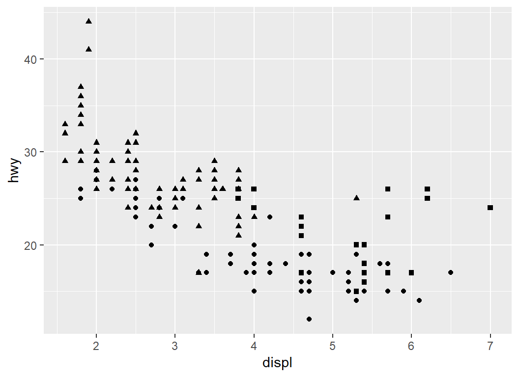
Illustration: remove legend
> p+theme(legend.position = "none")
Legend: remove fill for key
> # remove legend key background
> p + theme(legend.key = element_rect(fill=NA))
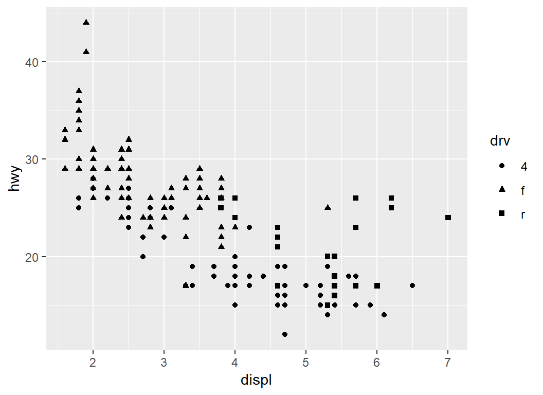
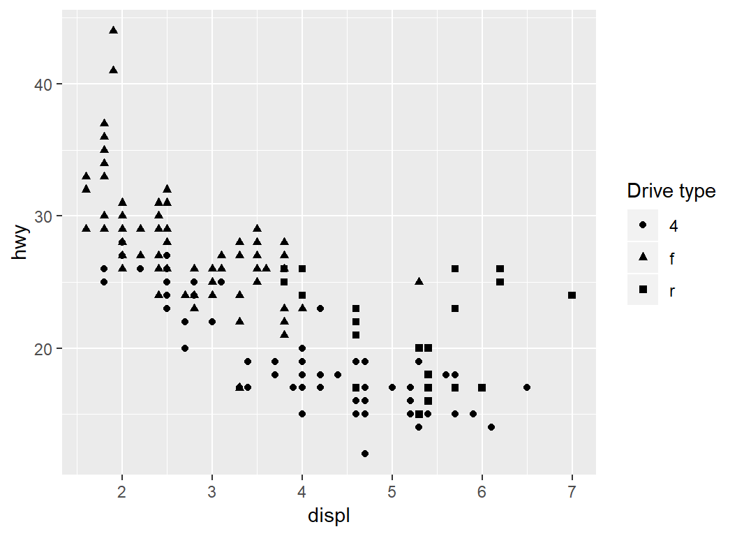
Illustration: change legend title
> # `shape` is the aesthetic and used by `labs`
> p+labs(shape = "Drive type")
Multiple legends
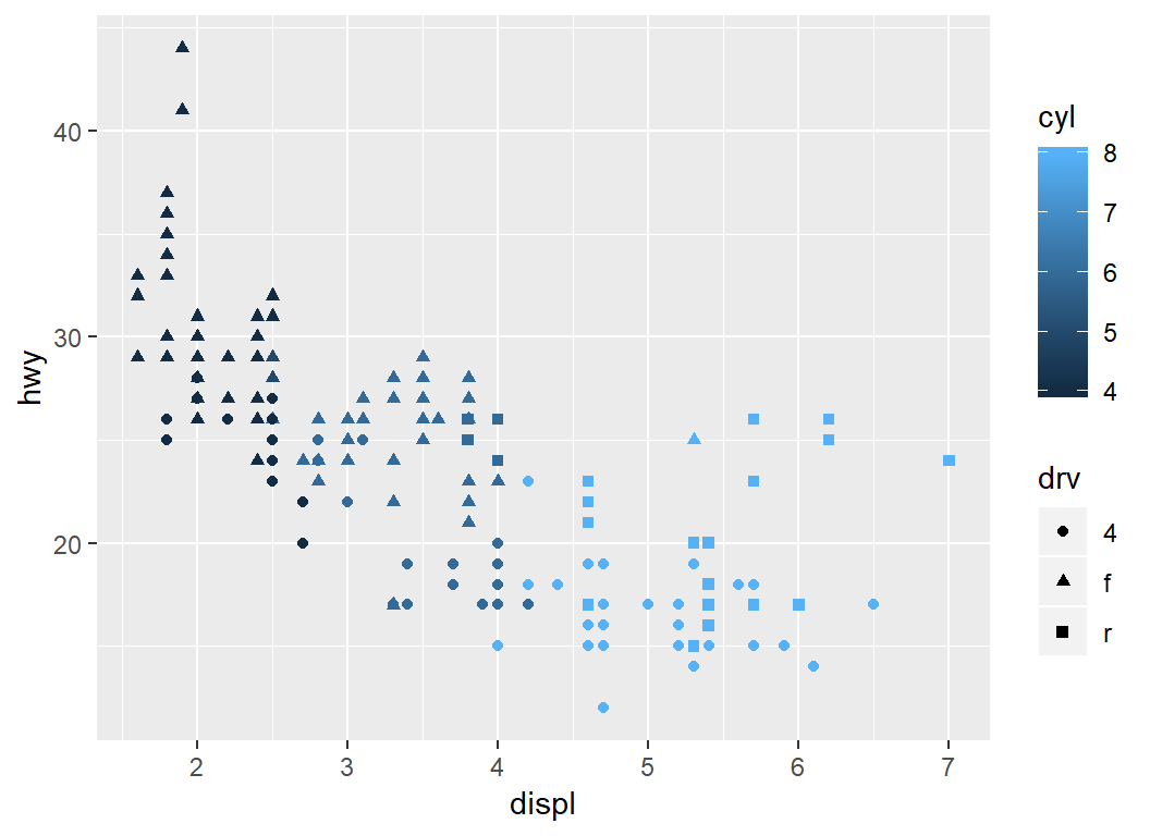
Plot displ vs hwy with color = cyl and shape=drv:
> library(ggplot2)
> p = ggplot(mpg, aes(displ,hwy))+
+     geom_point(aes(color = cyl, shape = drv))
- 2 legends will be created, one for
color and the other for shape
- by default, the 2 legends appear to the right of the plot and are aligned vertically
Multiple legends
> p
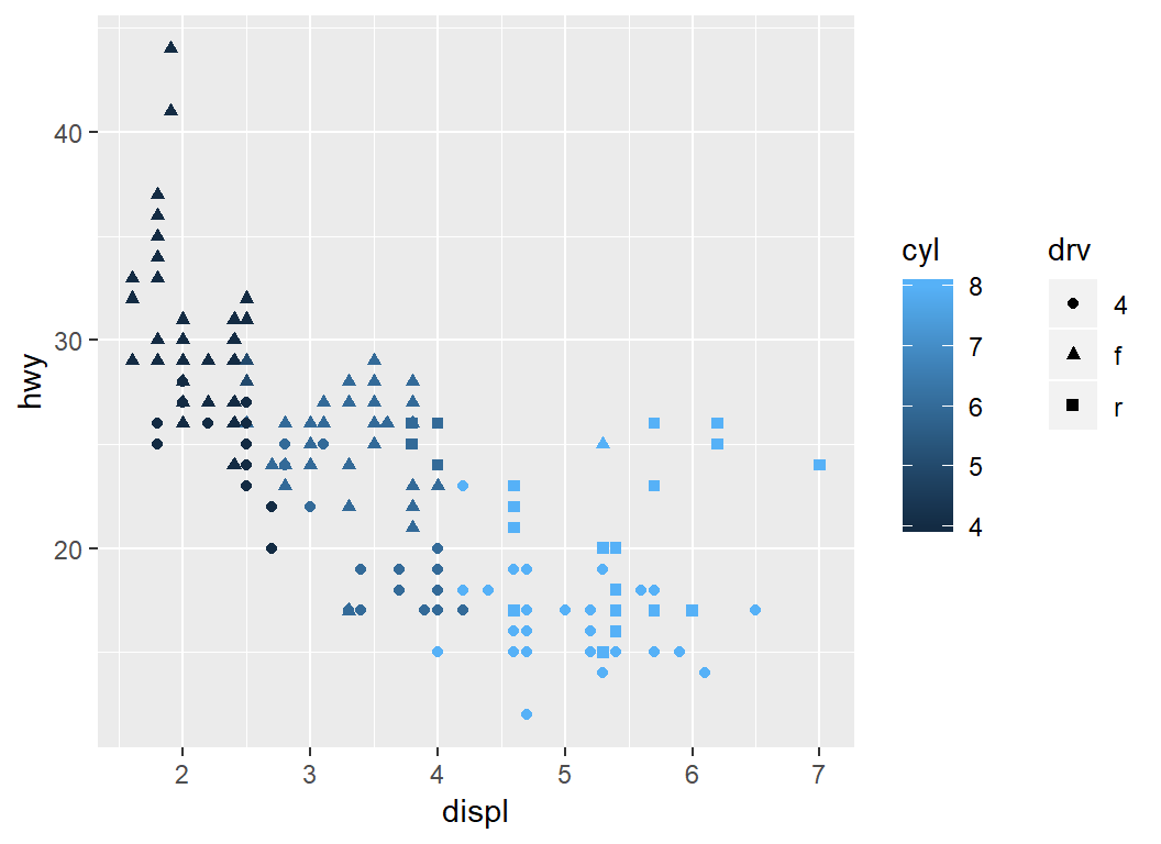
Multiple legends
> # Align the 2 legends horizontally
> p+theme(legend.box = "horizontal")
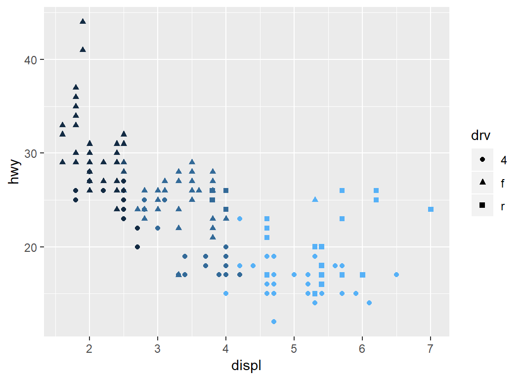
Hide a legend via guides
> # Hide legend for `color` via `guides`
> p + guides(color = FALSE)
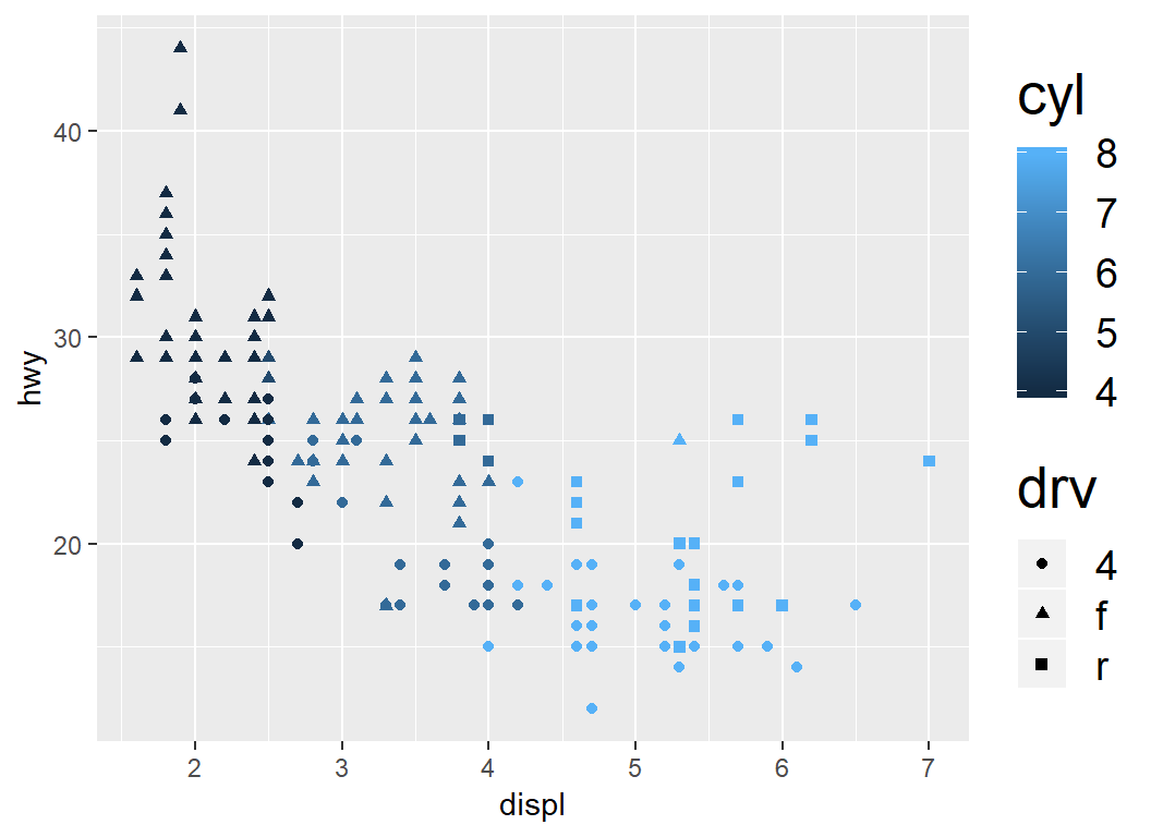
Legend text and title: font size
Brief synatx:
theme(
   legend.text=element_text(size=NULL),
  legend.title=element_text(size=NULL)
)
Replace NULL by a positive number
Legend: adjust font size
> p+theme(legend.text=element_text(size=14),
+   legend.title=element_text(size=20))
Adjusting font size and angle of text and label
Axis label and strip text
Brief syntax:
theme(
 axis.text.x =element_text(size=10,angle=0),
 axis.title.x =element_text(size=14,angle=30),
 axis.text.y =element_text(size=10,angle=0),
 axis.title.y =element_text(size=14,angle=-40),
 strip.text=element_text(size=12,angle=0)
 )
- “strip” appears when
facet_wrap or facet_grid is used, and it annotates the levels of variabels used for grouping
angle is used to rotate texts or labels; this is useful when texts or labels are long
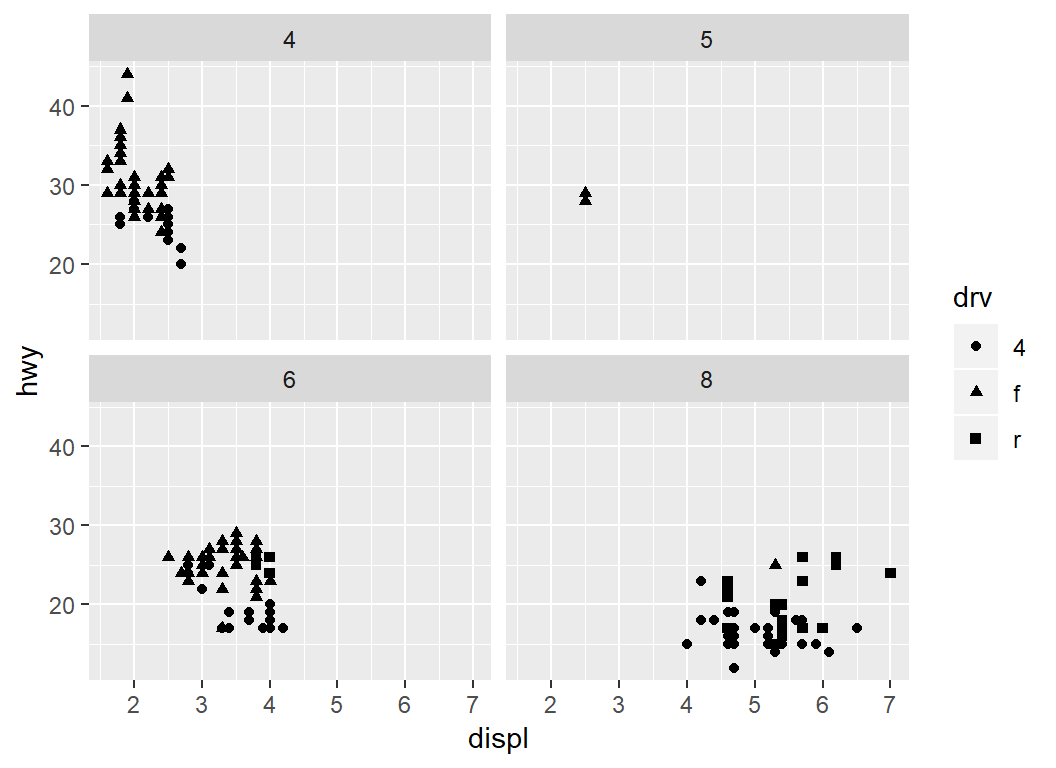
Illustration
Plot displ vs hwy with shape = drv and facet cyl:
> library(ggplot2)
> p = ggplot(mpg, aes(displ,hwy))+
+   geom_point(aes(shape = drv))+
+     facet_wrap(~cyl)
- by default, strip texts (i.e., facet labels) for
cyl are values of cyl
- by default, texts and labels follow default orientation
Illustration: default strip texts
> p
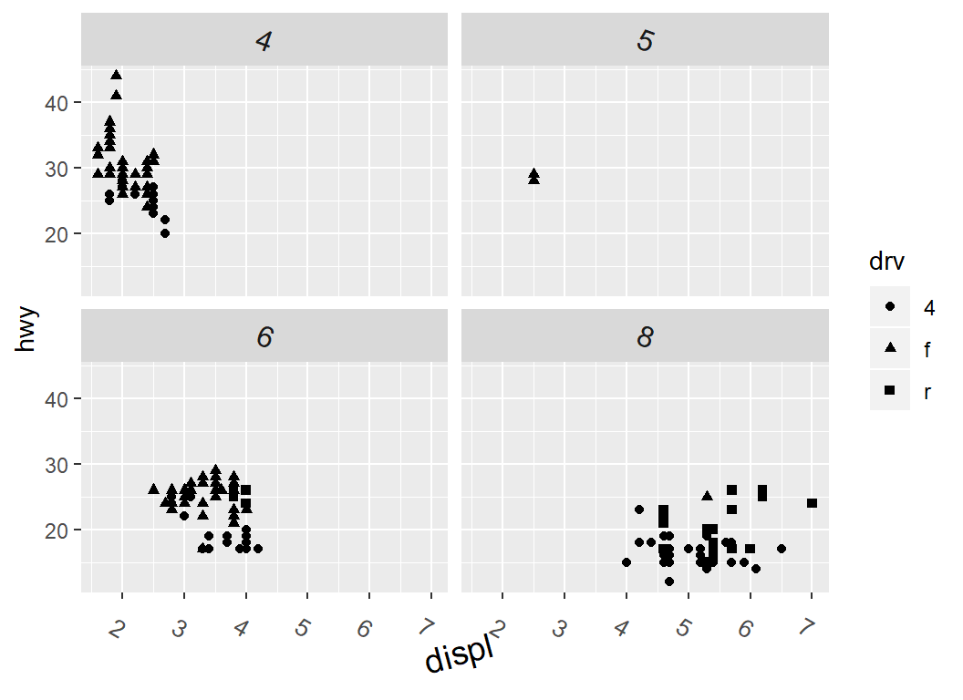
Adjust font size and orientation
> p + theme(axis.text.x =element_text(size=10,angle=-30),
+           axis.title.x =element_text(size=14,angle=15),
+           strip.text=element_text(size=12,angle = -20))
Overview
Math expressions do appear frequently in R plots. To show math expressions in plots, we
Create a mathematical expression
We will use
paste(..., sep = " ")
to create a string that contains plotmath syntax/commands, and
expression(...)
to convert it into a mathematical expression
plotmath syntax
plotmath shares some syntax/commands with latex. Here are some plotmath commands:
alpha, … , omega are for Greek symbols \(\alpha\), …, \(\omega\)x[y] represents \(x_{y}\), and x[y][z] represents \(x_{yz}\)x^2 represents \(x^2\)
Use demo(plotmath) to get more commands/syntax
The paste command
> paste("x", "trial", sep="")
[1] "xtrial"
>
> paste("x", "trial", sep=" ")
[1] "x trial"
sep="": no space between “x” and “trial” when they are concatenatedsep=" ": use a space to seperate “x” and “trial” when they are concatenated
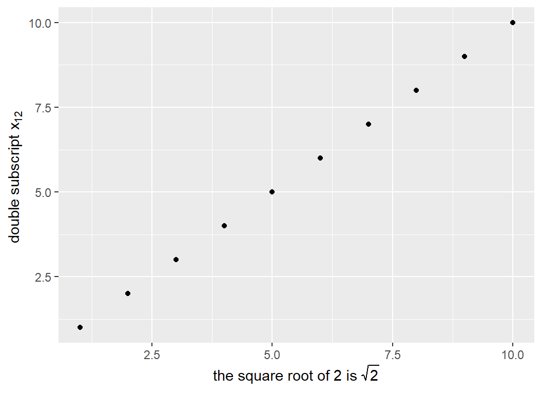
The expression command
> s1 = expression(paste("the square root of 2 is ",sqrt(2),
+                       sep=""))
> s2 = expression(paste("double subscript ", x[1][2],
+                       sep=" "))
> library(ggplot2)
> d1 = data.frame(cbind(1:10,1:10)); names(d1) = c("x1","y2")
> p10 = ggplot(d1,aes(x1,y2))+geom_point()+xlab(s1)+ylab(s2)
- “s1” is “the square root of 2 is \(\sqrt{2}\)”
- “s2” is “double subscript \(x_{12}\)”
- “s1” and “s2” are used as x-axis label and y-axis label respectively for plotting \((i,i)\) for \(i=1,\ldots,10\)
Unprocessed math expressions
> # view s1 and s2
> s1
expression(paste("the square root of 2 is ", sqrt(2), sep = ""))
> s2
expression(paste("double subscript ", x[1][2], sep = " "))
Note: the expressions “s1” and “s2” have not been processed when no plots that use them as labels are created
Math expressions in axis labels
> p10
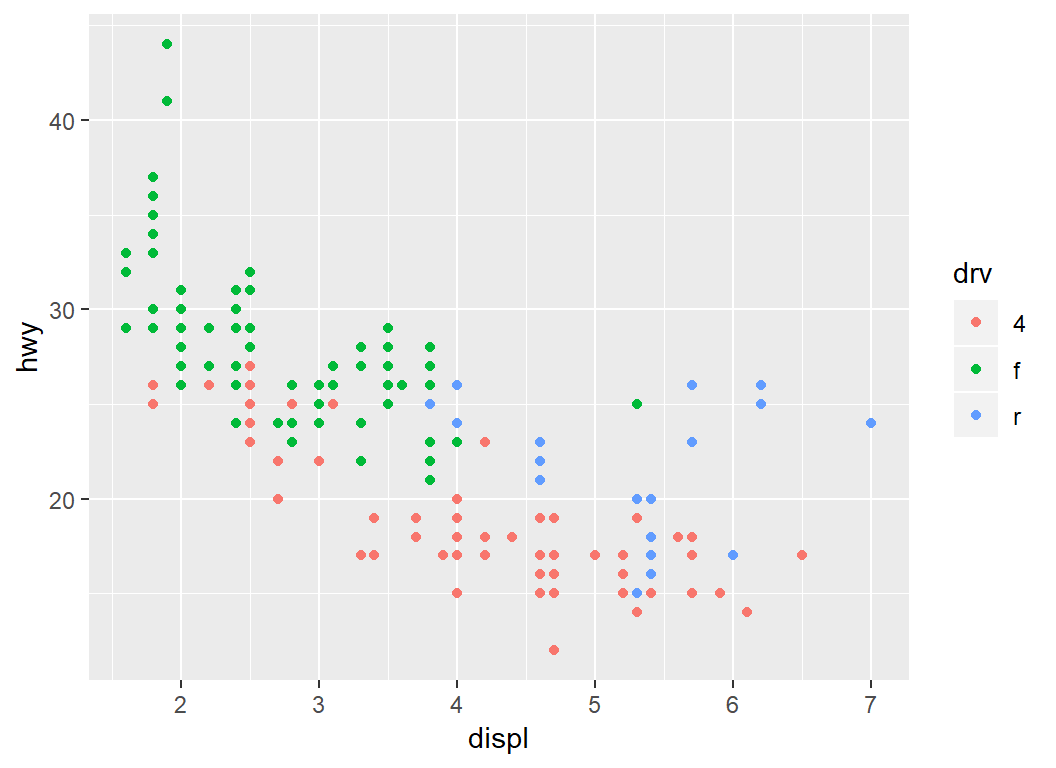
Math expression in legends
Plot displ vs hwy with coloring col = drv:
> library(ggplot2)
> p = ggplot(mpg, aes(displ,hwy))+geom_point(aes(col = drv))
drv has 3 levels “4”, “f” and “r”- the legend is created by
col, i.e., color or colour
- by default, key labels are levels of
drv
Math expression in legends
> p # note legend title and key labels
Math expression in legends
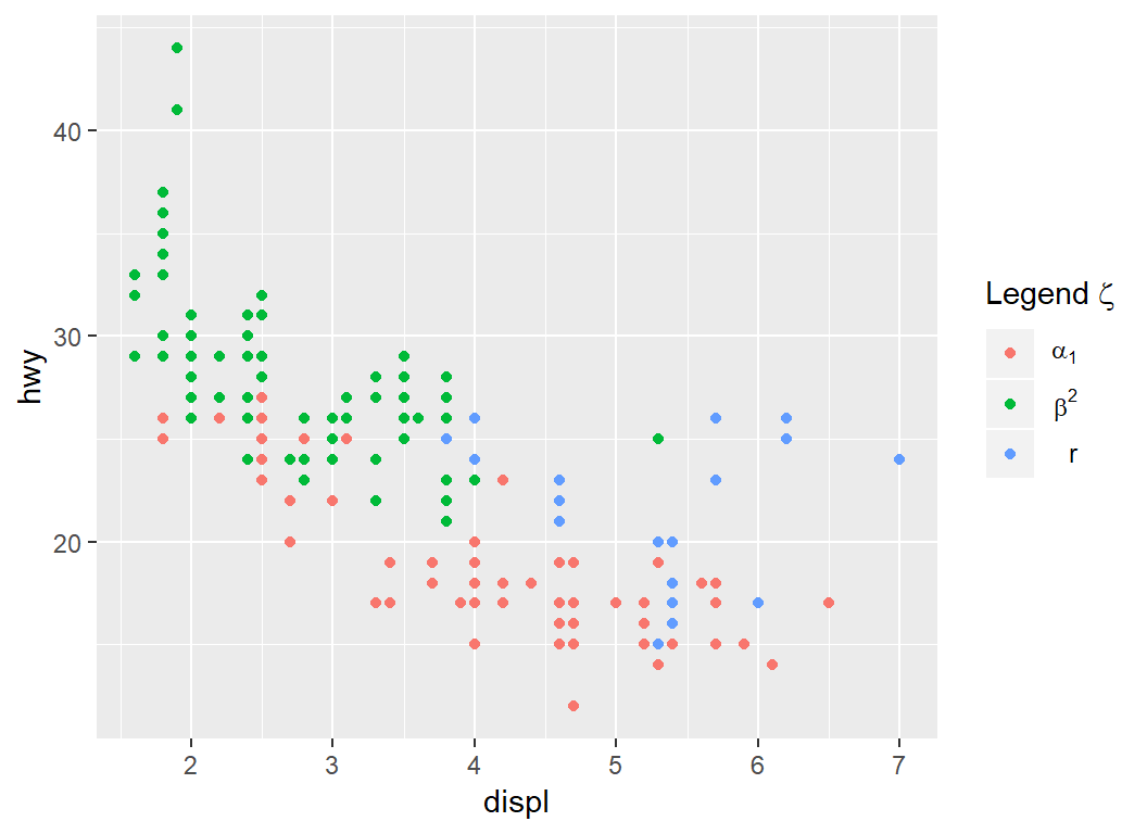
- map the 3 levels “4”, “f” and “r” of
drv to “\(\alpha_1\)”, “\(\beta^{2}\)” and “r”, respectively
- use “\(\alpha_1\)”, “\(\beta^{2}\)” and “r” as key labels for the legend created by
color aesthetic
- change legend title to “Legend \(\zeta\)”
> # map "4", "f" and "r" to expressions
> drvStg = c(expression(alpha[1]),expression(beta^2),
+            expression(r))
> # modify legend title
> p2c= p+labs(col=expression(paste("Legend ",zeta,sep="")))+
+ # modify legend key labels
+     scale_color_discrete(labels =drvStg)
Math expression in legends
> p2c
Math expression in strip texts
> library(ggplot2) # create based player
> p=ggplot(mpg,aes(displ,hwy))+geom_point()+facet_wrap(~drv);p

Math expression in strip texts
- map “4”, “f” and “r” to “\(\alpha_1\)”, “\(\beta^2\)” and “r”, respectively
- create variable
DF (a factor) with levels “\(\alpha_1\)”, “\(\beta^2\)” and “r”
- use
slice to check correctness of mapping
> drvStg = c(expression(alpha[1]),expression(beta^2),
+            expression(r))
> mpg$DF = factor(mpg$drv, labels =drvStg)
>
> library(dplyr)
> # check if the levels are labelled correctly
> mpg %>% select(displ, hwy, DF, drv) %>%
+   group_by(drv) %>% slice(1)
# A tibble: 3 x 4
# Groups:   drv [3]
  displ   hwy DF       drv
  <dbl> <int> <fct>    <chr>
1   1.8    26 alpha[1] 4
2   1.8    29 beta^2   f
3   5.3    20 r        r
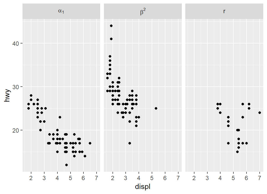
Math expression in strip texts
Create plot and
- use
labeller = label_parsed to parse expressions, which are levels of DF
- use parsed expressions as strip texts for
facet_wrap with DF:
> library(ggplot2)
> p5 = ggplot(mpg, aes(displ,hwy))+geom_point()+
+   facet_wrap(~DF,labeller = label_parsed)
Use ?ggplot2::labeller to get more information on labeller
Math expression in strip texts
> p5
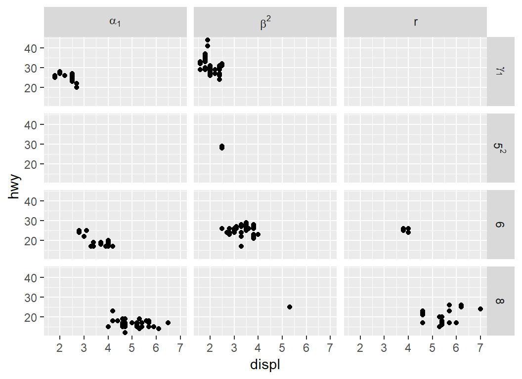
Parse expressions in strip texts
Math expressions in strip texts of facet_grid:
- map “4”, “5”, “6” and “8”, levels of
cyl, to “\(\gamma_1\)”, “\(5^2\)”, “6” and “8”, respectively
- create
CF (a factor) with levels “\(\gamma_1\)”, “\(5^2\)”, “6” and “8”
> cylStg = c(expression(gamma[1]),expression(5^2),"6","8")
> mpg$CF = factor(mpg$cyl, labels =cylStg)
> library(dplyr)
> # check if the levels are labelled correctly
> mpg %>% select(displ, hwy, CF, cyl) %>%
+         group_by(cyl) %>% slice(1)
# A tibble: 4 x 4
# Groups:   cyl [4]
  displ   hwy CF         cyl
  <dbl> <int> <fct>    <int>
1   1.8    29 gamma[1]     4
2   2.5    29 5^2          5
3   2.8    26 6            6
4   4.2    23 8            8
Parse expressions in strip texts
> # parse expressions for both faceting variables
> ggplot(mpg, aes(displ,hwy))+geom_point()+
+   facet_grid(CF~DF,labeller = label_parsed)
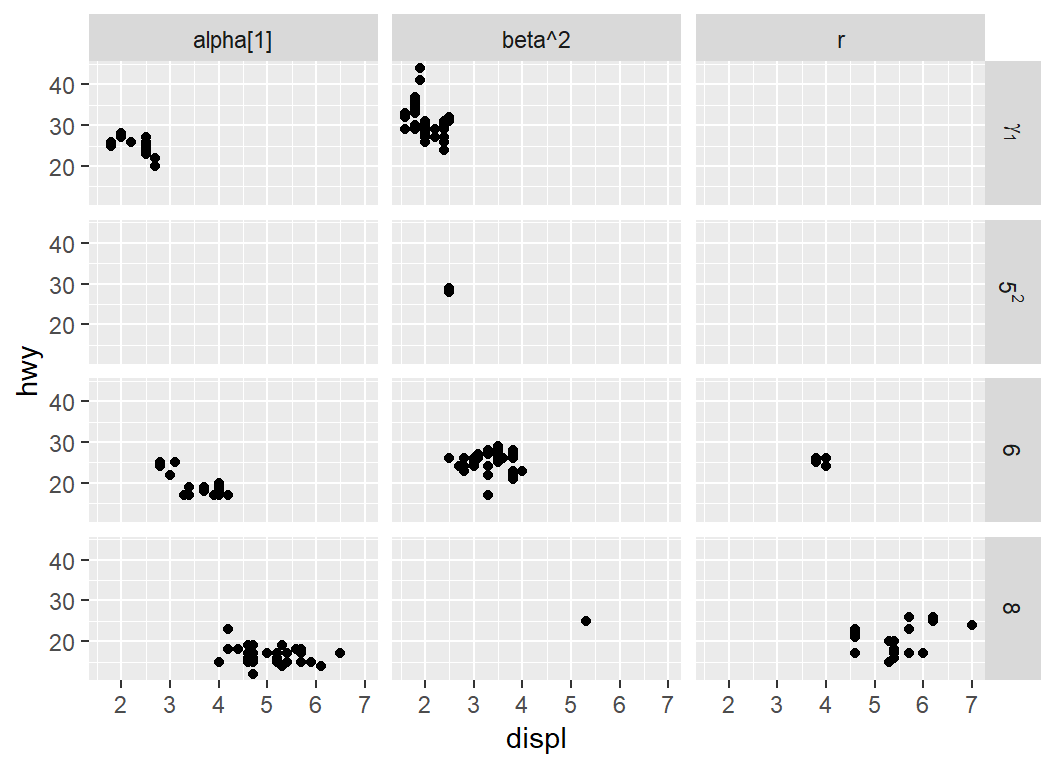
Parse expressions in strip texts
> # parse expression for `CF` only
> ggplot(mpg, aes(displ,hwy))+geom_point()+
+   facet_grid(CF~DF,labeller = labeller(CF=label_parsed))
A few other ggplot2 twicks
geom_ + scale*manual
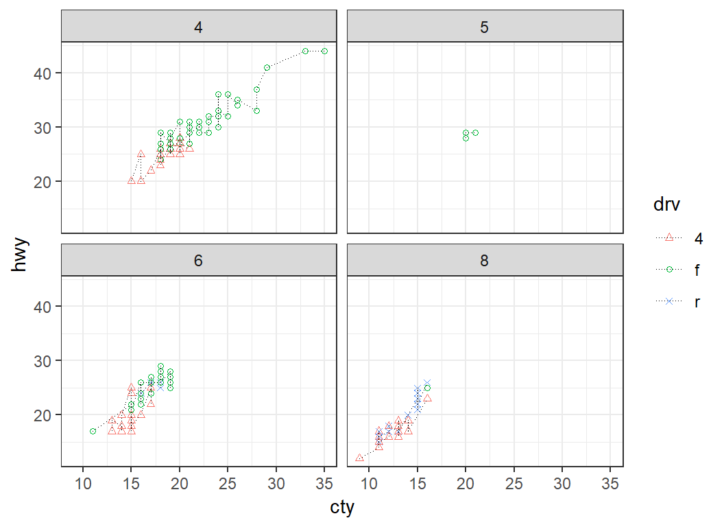
Manually specify shapes and line types:
> library(ggplot2)
> p5 = ggplot(mpg, aes(cty,hwy))+ facet_wrap(~cyl)+theme_bw()+
+   geom_point(aes(shape = drv,color=drv),size=1.2) +
+   scale_shape_manual(values=c(2,1,4))+
+   geom_line(aes(linetype = drv),size=0.3)+
+   scale_linetype_manual(values=rep("dotted",3))
geom_point+scale_shape_manual: manually specify shapes; points are assigned shapesgeom_line+scale_linetype_manual: manually specify line types: points are connected by linesshape = drv,color=drv and linetype = drv: 3 legends as 1 and by drv
geom_ + scale*manual
> p5
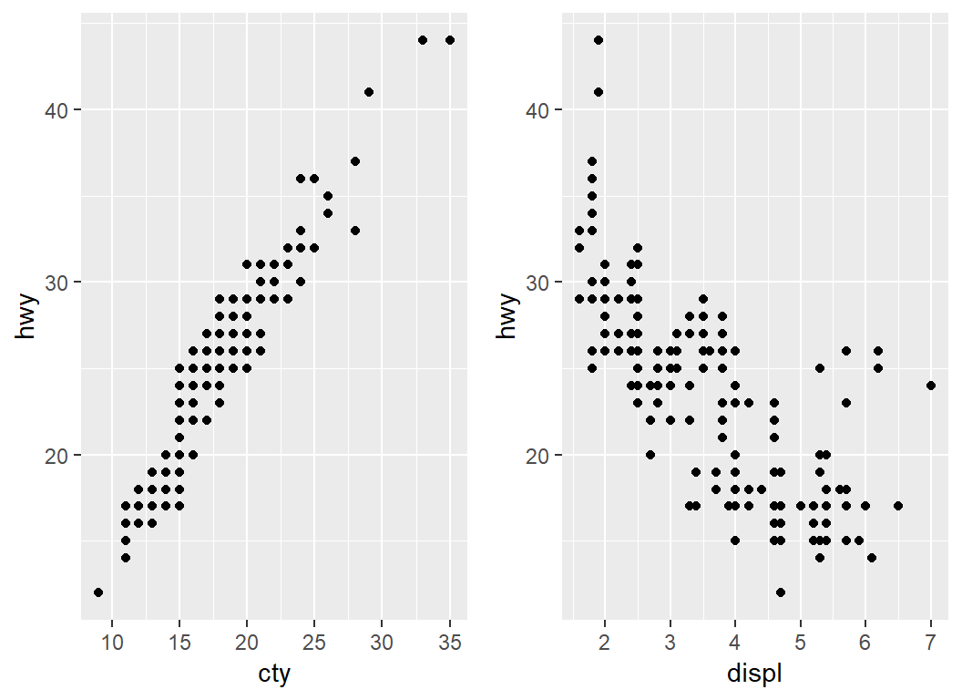
Combine ggplot2 plots
The R packages grid and gridExtra can be used to combined two or more ggplot2 plots
> # create 2 plots
> p1 = ggplot(mpg, aes(cty,hwy))+geom_point()
> p2 = ggplot(mpg, aes(displ,hwy))+geom_point()
Combine ggplot2 plots
> # combine p1 and p2 into one plot and put them in a row
> library(gridExtra); grid.arrange(p1,p2,nrow=1)
Not covered
The following have not been covered:
- some statistical transforms:
stat_XXX
- figure margin adjustment:
margin
Information on the above can be found in the book “ggplot2: elegant graphs for data analysis” by Hadley Wickham, or in various online resources
