Clustering: motivation

Clustering is widely applied:

• Marketing: consumers can be split into groups (according to their preferences) for better product positioning
• Medicine: antibiotics can be split into groups (according to their antibacterial activities) for better treatment of patients
• Economics: stocks can be split into groups (according to their economic divisions) for better regulation

Clustering is often used in exploratory data analysis or as a starting point of further study.

Clustering: basic principle

In general, clustering refers to a broad set of techniques for finding subgroups or, clusters, in a data set.

In principle, clustering divides data into groups, such that

• Observations within each group are quite similar to each other
• Observations in different groups are quite different from each other

Clustering depends on the concept of “similarity” (or “dissimilarity”) (to be introduced later).

Two clustering methods

We will discuss two clustering methods:

• K-means clustering
• Hierarchical clustering

Two books

• The “thin” book (as the Text): “An introduction to statistical learning with applications in R”, by Gareth James. Daniela Witten. Trevor Hastie. Robert Tibshirani. Available free at https://faculty.marshall.usc.edu/gareth-james/ISL/

• The “thick” book (as reference): “The Elements of Statistical Learning: Data Mining, Inference, and Prediction, 2nd Ed.”, by T. Hastie, R. Tibshirani and J. Friedman. Available free at https://web.stanford.edu/~hastie/ElemStatLearn/

Materials and organization

Learning unit on K-means uses:

1. Sections 10.3.1 and 10.5.1 of the Text
2. R commands and libraries:

• R command kmeans for K-means clustering
• The function clusGap from library cluster (to estimate the number of clusters in data)
• R library ElemStatLearn (which provides example data sets)

Learning unit has 3 parts: methodology, practical issues, and software implementation

Feature vector and observations

The “Iris” data set (from the library ggplot2) contains 150 measurements of 4 features for Iris flowers:

  Sepal.Length Sepal.Width Petal.Length Petal.Width
1          5.1         3.5          1.4         0.2
2          4.9         3.0          1.4         0.2
3          4.7         3.2          1.3         0.2

• Features: \(x_1\) =Sepal.Length, \(x_2\)=Sepal.Width, \(x_3\)=Petal.Length, \(x_4\)=Petal.Width
• Feature vector: \(\boldsymbol{x} = (x_1,x_2,x_3,x_4),\) a \(4\)-vector, i.e., feature dimension \(p=4\)
• Observation \(i\) for \(\boldsymbol{x}\): \(\boldsymbol{x}_i = (x_{i1},x_{i2},x_{i3},x_{i4})\); e.g., \(\boldsymbol{x}_1 = (x_{11},x_{12},x_{13},x_{14}) = (5.1,3.5,1.4,0.2)\); \(\boldsymbol{x}_2 = (x_{21},x_{22},x_{23},x_{24}) = (4.9,3.0,1.4,0.2)\)

Euclidean distance

The Euclidean distance between two observations \(\boldsymbol{x}_i=(x_{i1},\ldots,x_{ip})\) and \(\boldsymbol{x}_j=(x_{j1},\ldots,x_{jp})\) of the \(p\)-dimensional feature vector \(\boldsymbol{x}\): \[d(\boldsymbol{x}_i,\boldsymbol{x}_{j}) = \left(\sum_{k=1}^p (x_{ik} - x_{jk})^2\right)^{1/2}\]

• \(\boldsymbol{x}_1 = (5.1,3.5,1.4,0.2)\); \(\boldsymbol{x}_2 = (4.9,3.0,1.4,0.2)\)

> x1 = c(5.1,3.5,1.4,0.2); x2 = c(4.9,3.0,1.4,0.2)
> # compute Euclidean distance
> d = sqrt(sum((x1-x2)^2))
> d
[1] 0.5385165

Dissimilarity measure

• The dissimilarity between \(\boldsymbol{x}_i\) and \(\boldsymbol{x}_{j}\) is defined as \[d_{ij} = d^2(\boldsymbol{x}_i, \boldsymbol{x}_{j}),\] where \(d\) is the Euclidean distance.

• Smaller \(d_{ij}\) means \(\boldsymbol{x}_i\) and \(\boldsymbol{x}_{j}\) are more similar and less dissimilar.

> x1 = c(5.1,3.5,1.4,0.2); x2 = c(4.9,3.0,1.4,0.2)
> x3 = c(4.7,3.2,1.3,0.2)
> # Euclidean distance between x1 and x2
> sqrt(sum((x1-x2)^2))
[1] 0.5385165
> # Euclidean distance between x1 and x3
> sqrt(sum((x1-x3)^2))
[1] 0.509902

Clustering as a mapping

\(K\)-means clustering divides observations into \(K\) disjoint clusters and assigns each observation to a cluster. For example:

• When \(K=2\), each observation will be assigned to one of 2 disjoint clusters, Cluster 1 or Cluster 2
• Let \(k=1\) or \(2\) denote the cluster membership of an observation

Clustering can be regarded as a mapping \(C\) that assigns the \(i\)th observation \(\boldsymbol{x}_i\) to Cluster \(k\). However, how the clusters are numbered is arbitrary as long as there are \(K\) disjoint clusters.

Centroids and variability

• Let \(N_k\) be the number of observations in Cluster \(k\)

• The centroid for Cluster \(k\) is defined as \[ \bar{\boldsymbol{x}}_{k} = \frac{1}{N_k} \sum_{ \left\{ \boldsymbol{x}_i \text{ in Cluster } k \right\}} \boldsymbol{x}_i \] Namely, the centroid for Cluster \(k\) is the sample mean of its observations

• The sample variance of observations in Cluster \(k\) is \[ S_k^2 = \frac{1}{N_k} \sum_{ \left\{ \boldsymbol{x}_i \in \text{ in Cluster } k \right\} } d^2(\boldsymbol{x}_i, \bar{\boldsymbol{x}}_k) \]

Loss function for K-means

• Recall clustering, as a mapping \(C\), creates clusters for which observations within a cluster are quite similar but those between clusters are quite dissimilar.
• Recall Smaller \(d(\boldsymbol{x}_i,\boldsymbol{x}_j)\) for observations \(\boldsymbol{x}_i\) and \(\boldsymbol{x}_{j}\) means they are more similar and less dissimilar.

It can be shown that, when \(K=2\), \(K\)-means attempts to minimize the “loss function”: \[ W(C) = \sum_{ \left\{ \boldsymbol{x}_i \text{ in Cluster } 1 \right\} } d^2(\boldsymbol{x}_i, \bar{\boldsymbol{x}}_1)+ \sum_{ \left\{ \boldsymbol{x}_i \text{ in Cluster } 2 \right\} } d^2(\boldsymbol{x}_i, \bar{\boldsymbol{x}}_2) \]

Interpretation of the loss

In general, \(K\)-means attempts to minimize the loss function: \[ \begin{aligned} W(C) &= \sum_{k=1}^K \sum_{ \left\{ \boldsymbol{x}_i \text{ in Cluster } k \right\} } d^2(\boldsymbol{x}_i, \bar{\boldsymbol{x}}_k)\\ & = N_1 \times S_1^2 + \cdots + N_K \times S_K^2 \end{aligned} \]

• Each summand is the within-cluster variability (or within-cluster sum of squares) for the corresponding cluster (and equals to \(N_k \times\) sample variance of Cluster \(k\))

Namely, K-means attempts to minimize the total within-cluster variability (i.e.,total within-cluster sum of squares or total within-cluster dissimilarity)

An algorithm for K-means

\(K\)-means can be implemented by the following Algorithm:

1. Randomly assign a number, from \(1\) to \(K\), to each observation, as its initial cluster membership.
2. Iterate the following 2 substeps until the cluster assignments stop changing:

• (2.a) For each cluster, compute the cluster centroid.
• (2.b) Assign each observation to the cluster whose centroid is closest (in Euclidean distance).

Note: When the cluster assignments stop changing, we say that the “Algorithm converges” (perhaps only to a local minimum of the loss function).

Quick visualization of Algorithm

The “Iris” data set (from the library ggplot2) contains measurements of 4 features for 150 Iris flowers for 3 Spieces of Iris:

  Sepal.Length Sepal.Width Petal.Length Petal.Width Species
1          5.1         3.5          1.4         0.2  setosa
2          4.9         3.0          1.4         0.2  setosa
3          4.7         3.2          1.3         0.2  setosa
4          4.6         3.1          1.5         0.2  setosa
5          5.0         3.6          1.4         0.2  setosa
6          5.4         3.9          1.7         0.4  setosa

We will visualize the Algorithm by clustering the observations into \(4\) clusters using 2 features Sepal.Length and Sepal.Width.

Quick visualization of Algorithm

Cluster centroids and/or assignments evolve with iteration until convergence:

On the K-means Algorithm

• Under any initial configuration (in terms of initial cluster memberships), the algorithm always converges to a local minimum of the loss function, even though it is not ensured to converge to the global minimum of the loss function

• Different initial configurations for the Algorithm may give different clustering results when it converges

• The Algorithm needs to run under multiple initial configurations to help get closer to the global minimum of the loss function by choosing a best initial configuration

On dissimilarity measure

The previous K-means methodology employs the squared Euclidean distance as a dissimilarity measure. This

• reduces computational complexity, but
• places large influences on large distances, thus reducing the robustness of the methodology against outliers

The squared Euclidean distance is not the only available dissimilarity measure (that K-means can use).

Dissimilarity I

For two observations \(\boldsymbol{x}_i=(x_{i1},\ldots,x_{ip})\) and \(\boldsymbol{x}_j=(x_{j1},\ldots,x_{jp})\) of \(p\) quantitative features, their dissimilarity can also be defined as:

• Correlation distance: \(1- corr(\boldsymbol{x}_i,\boldsymbol{x}_j)\), where \(corr\) is the Pearson correlation between the \(p\) samples \((x_{ik},x_{jk}),k=1,\ldots,p\) (i.e., the \(p\) paired entries of \(\boldsymbol{x}_i\) and \(\boldsymbol{x}_j\))
• Manhattan distance: \(\sum_{k=1}^p \vert x_{ik} - x_{jk}\vert\) (i.e., the sum of absolute differences between the \(p\) paired entries of \(\boldsymbol{x}_i\) and \(\boldsymbol{x}_j\))

Dissimilarity II

For observations for qualitative features, dissimilarity can be defined by first mapping each value in the range into a numerical value, and then work on the transformed values:

• Ordinal variable (such as academic grades): let \(M\) be the total number of ordinal values the variable can assume, and \(y\) be the observed value; then \[y \mapsto \tilde{y}=[\textrm{rank}(y) - 2/M]/M\]

• Nominal variable (such as gender): for values \(a\) and \(b\) in the range of the variable, set \(d(a,b) = 0\) when \(a=b\) and \(d(a,b) = 1\) when \(a \ne b\)

The true number of clusters

In practice, the true number \(K_0\) of clusters for data is unknown and needs to be estimated. For this,

• The “gap statistic” can be used, is based on differences between within-cluster sums of squares, and is implemented by the function clusGap of the library cluster

Caution: the gap statistic does not estimate \(K_0\) correctly for each data set. Instead, a set of assumptions should be satisfied to ensure its accuracy.

Required commands and software

R software and commands required:

• Library ElemStatLearn which contains example data sets
• Command kmeans to implement the Algorithm for k-means
• Library cluster and its function clusGap to estimate the number of clusters in data

Command: kmeans

Basic syntax:

kmeans(x, centers, iter.max = 10, nstart = 1,algorithm = 
        c("Hartigan-Wong", "Lloyd", "Forgy","MacQueen"))

• x: data object as a matrix; \(i\)th observation as the \(i\)th row
• centers: number \(K\) of clusters to form, or a matrix containing centroids
• nstart: number of random, initial configurations of cluster memberships
• algorithm: algorithm to minimize the loss function; “Hartigan-Wong” as the default
• iter.max: maximum of number of iterations run by algorithm, with default as 10

Command: kmeans

kmeans command returns

• cluster: a vector of integers (from \(1\) to \(K\)), the value \(k_i\) of whose \(i\)th entry indicates that the \(i\)th observation is assigned to Cluster \(k_i\), where \(K\) is the number of clusters to form
• centers: a matrix of cluster centers (i.e., centroids), whose \(j\)th row contains the coordinates of the centroid of Cluster \(j\)
• tot.withinss: total within-cluster sum of squares

Cautions on kmeans

1. Data x must contain the \(i\)th observation of features in its \(i\)th row
2. kmeans cannot be applied to non-numerical data x
3. Even with the same number \(K\) of clusters to form from x,

• different nstart values may give different clustering results since K-means algorithm may converge to different local optima of the loss function under different initial configurations
• different iter.max values may give different clustering results since intermediate results of K-means algorithm may differ at different iterations (before it converges to any local optimum of the loss function)

Generate Gaussian data

Codes to generate data:

> set.seed(2); x=matrix(rnorm(50*2), ncol=2)
> x[1:25,1]=x[1:25,1]+3; x[1:25,2]=x[1:25,2]-4

• Data have \(N=50\) observations, each for for \(2\) features, and are stored in a \(50 \times 2\) matrix (such that each row is an observation)
• The 1st \(25\) observations are bivariate Gaussian with mean vector \(\boldsymbol{\mu}_1=(3,-4)\) and identity covariance matrix \(\boldsymbol{I}_2\)
• The rest \(25\) observations are bivariate Gaussian with mean vector \(\boldsymbol{\mu}_2=(0,0)\) and identity covariance matrix \(\boldsymbol{I}_2\)

Observations form 2 clusters (or groups) if we assign them according to their 2 different mean vectors.

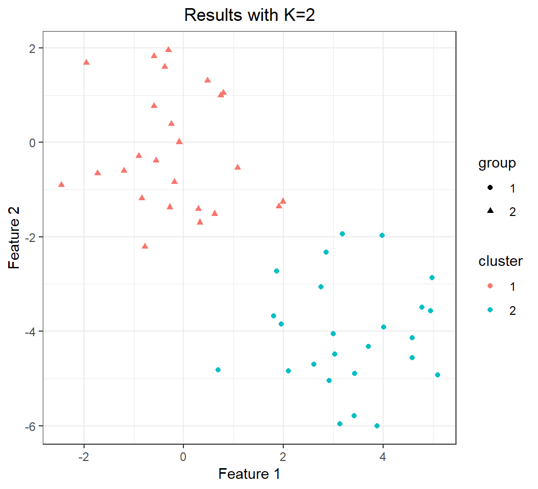
Effect of K: K=2

Split observations into \(K=2\) clusters:

> km.out=kmeans(x,2,nstart=20)
> # creat new data.frame with "group" and "cluster"
> y = data.frame(x); colnames(y)=c("X1","X2")
> y$group = factor(rep(c(1,2),each=25))
> y$cluster=factor(km.out$cluster)
> library(ggplot2)
> p = ggplot(y,aes(X1,X2))+
+   geom_point(aes(shape=group,color=cluster))+
+   xlab("Feature 1")+ylab("Feature 2")+
+   ggtitle("Results with K=2")+theme_bw()+
+   theme(plot.title = element_text(hjust = 0.5))

• group: cluster membership determined by mean vectors
• cluster: cluster membership given by K-means

Perfect clustering is achieved when group matches cluster

Effect of K: K=2

Perfect clustering (compared to truth):

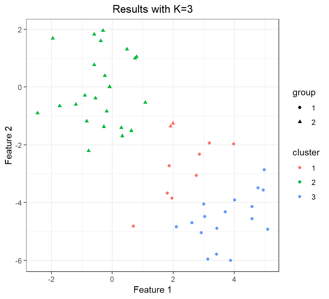
Effect of K: K=3

Split observations into \(K=3\) clusters:

> set.seed(4); km.out3 =kmeans(x,3,nstart=20)
> # show the 3 centroids
> km.out3$centers
        [,1]        [,2]
1  2.3001545 -2.69622023
2 -0.3820397 -0.08740753
3  3.7789567 -4.56200798
> # creat new data.frame with "group" and "cluster"
> y = data.frame(x); colnames(y)=c("X1","X2")
> y$group = factor(rep(c(1,2),each=25))
> y$cluster=factor(km.out3$cluster)
> library(ggplot2)
> p = ggplot(y,aes(X1,X2))+
+   geom_point(aes(shape=group,color=cluster))+
+   xlab("Feature 1")+ylab("Feature 2")+
+   ggtitle("Results with K=3")+theme_bw()+
+   theme(plot.title = element_text(hjust = 0.5))

Note: there are only two clusters in the data.

Effect of K: K=3

Bad clustering (compared to truth):

Effect of “nstart”

• nstart controls the number of random, initial configurations of cluster memberships for the K-means algorithm, and kmeans only reports results from the best configuration (determined in terms of loss, i.e., total within-cluster sum of squares).

• nstart is recommended to be large, such as 20 or 50

> set.seed(2); x=matrix(rnorm(50*2), ncol=2)
> x[1:25,1]=x[1:25,1]+3; x[1:25,2]=x[1:25,2]-4
> set.seed(3)
> km.out=kmeans(x,3,nstart=1)
> km.out$tot.withinss
[1] 104.3319
> km.out=kmeans(x,3,nstart=20)
> km.out$tot.withinss
[1] 97.97927

Effect of “set.seed”

K-means algorithm uses a random initialization. So, to make the kmeans results replicable, set.seed() should be used (to make reproducible the random initialization) before running kmeans.

In summary, a good practice is:

set.seed(123)
kmeans(x, ...)

where 123 in set.seed() can be another real number

A quick look at data

The “iris” data set (included in the library ggplot2) has measurements in centimeters of 4 features for 50 Iris flowers from each of 3 Species of Iris, i.e., setosa, versicolor, and virginica.

> library(ggplot2)
> head(iris)
  Sepal.Length Sepal.Width Petal.Length Petal.Width Species
1          5.1         3.5          1.4         0.2  setosa
2          4.9         3.0          1.4         0.2  setosa
3          4.7         3.2          1.3         0.2  setosa
4          4.6         3.1          1.5         0.2  setosa
5          5.0         3.6          1.4         0.2  setosa
6          5.4         3.9          1.7         0.4  setosa

Observations form 3 clusters if we insist on their associated 3 species.

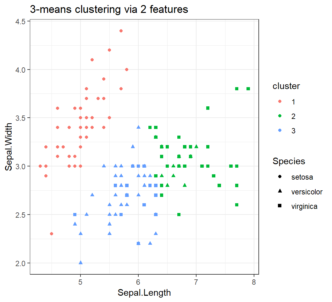
Clustering via 2 features

Split data into 3 clusters via 2 features Sepal.Length and Sepal.Width:

> library(ggplot2); set.seed(3.14)
> # use `Sepal.Length` and `Sepal.Width`
> km.out=kmeans(iris[,1:2],3,nstart=20)
> # augment "iris" with "cluster"
> iris$cluster=factor(km.out$cluster)
> library(ggplot2)
> p = ggplot(iris,aes(Sepal.Length,Sepal.Width))+
+   geom_point(aes(shape=Species,color=cluster))+
+   theme_bw()+ggtitle("3-means clustering via 2 features")

• Species: cluster membership determined by Species
• cluster: cluster membership given by K-means

Caution: Species is not a feature and cannot be used by kmeans for clustering.

Clustering via 2 features

3 clusters via Sepal.Length and Sepal.Width:

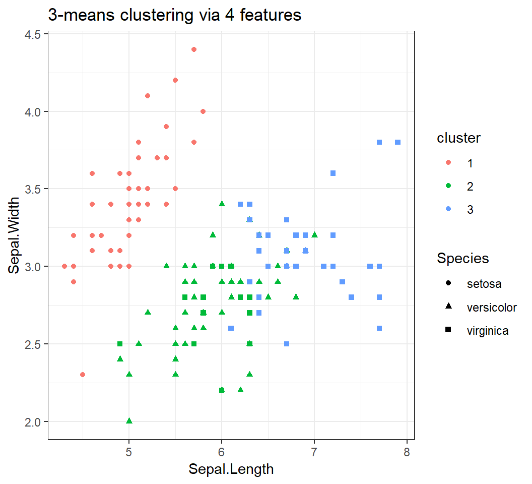
Clustering via 4 features

3 clusters via all 4 features:

> library(ggplot2); set.seed(3.14)
> # use `Sepal.Length` and `Sepal.Width` but not "Species"
> km.out=kmeans(iris[,1:4],3,nstart=20)
> # augment "iris" with "cluster"
> iris$cluster=factor(km.out$cluster)
> library(ggplot2)
> p1 = ggplot(iris,aes(Sepal.Length,Sepal.Width))+
+   geom_point(aes(shape=Species,color=cluster))+
+   theme_bw()+ggtitle("3-means clustering via 4 features")

• Species: underlying cluster membership
• cluster: cluster membership given by K-means

For simplicity but without losing information on clustering, we will use 2 features to track observations in visualizing clustering results even though 4 features are used.

Clustering via 4 features

3 clusters via 4 features:

A comparison

> library(gridExtra); grid.arrange(p,p1,nrow=1)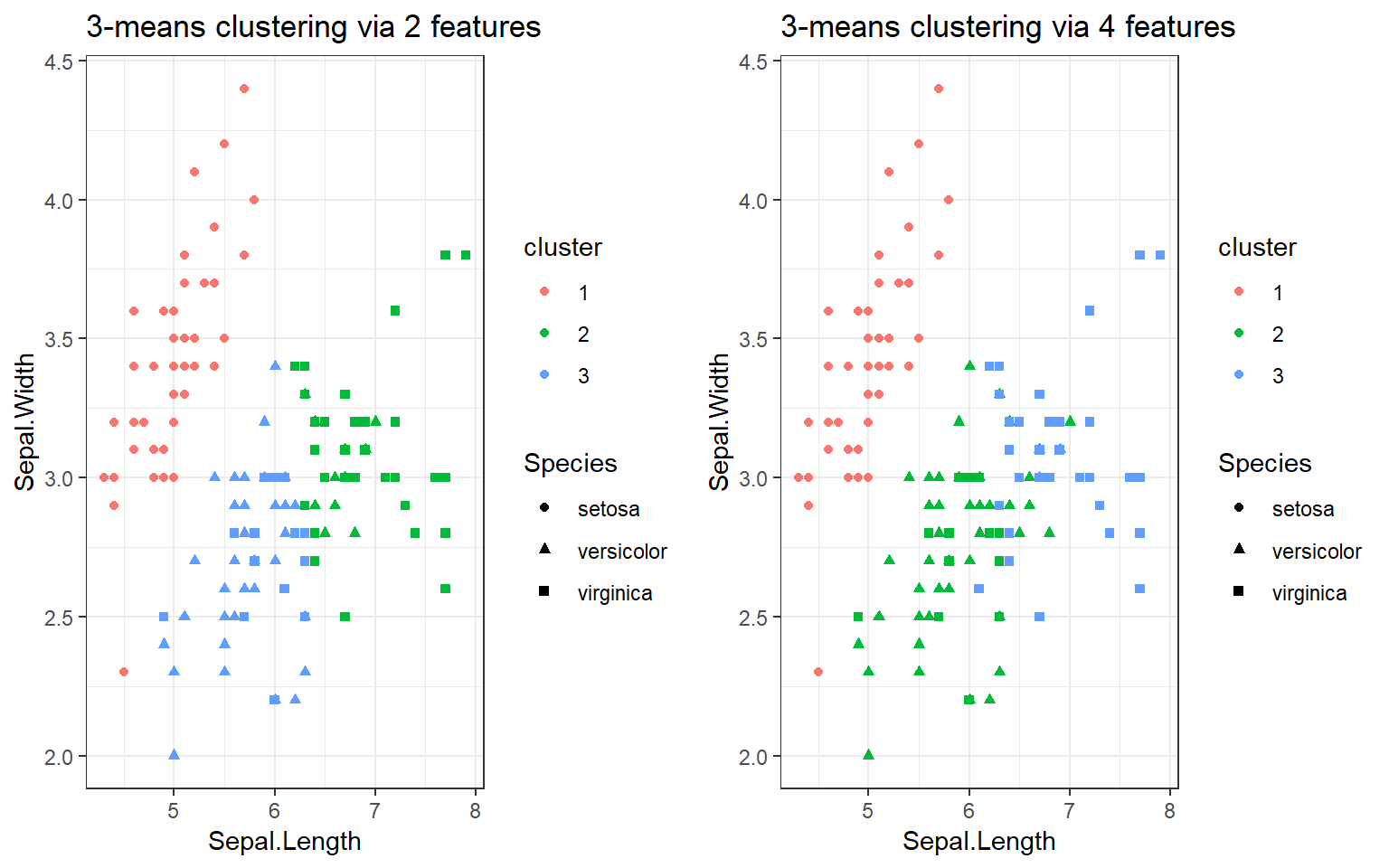

> # Note: cluster numbering is non-essential

Implement “gap statistic”: I

The gap statistic is implemented by the function clusGap in the library cluster. The basic syntax for clusGap is:

clusGap(x, FUNcluster, K.max, B = 100, 
        iter.max = 10, nstart=20)

• x is data set, and FUNcluster is set as kmeans
• K.max: maximum number of clusters to consider; must be at least two
• B: number of Monte Carlo (“bootstrap”) samples; larger B, more computation
• iter.max and nstart: same as those for kmeans

Note: clusGap accepts most arguments of kmeans

Implement “gap statistic”: II

clusGap returns Tab (accessible via $):

• Tab: a matrix with K.max rows and 4 columns, named “logW”, “E.logW”, “gap”, and “SE.sim”
• Tab[, "gap"]: vector of gap statistics, each of whose entries is for a different number of clusters
• Tab[, "SE.sim"]: vector of standard errors for entries of Tab[, "gap"]; \(i\)th entry of Tab[, "SE.sim"] is for \(i\)th entry of Tab[, "gap"]; “SE.sim” is obtained by bootstrapping

Implement “gap statistic”: III

Once clusGap has been executed, say, with return gapEst as in gapEst = clusGap(...), we can estimate the true number \(K_0\) of clusters by executing

maxSE(f, SE.f,
      method = c("firstSEmax", "Tibs2001SEmax", 
      "globalSEmax", "firstmax", "globalmax"),
      SE.factor = 1)

• f= gapEst$Tab[, "gap"] and SE.f= gapEst$Tab[, "SE.sim"] are set
• method: method to use to determine \(K_0\); default is “firstSEmax” but “Tibs2001SEmax” is recommended
• SE.factor= 1: the “one standard error (1-SE)” rule

Illustration of gap statistic

Estimate the true number \(K_0\) of clusters of iris data using 2 features Sepal.Length and Sepal.Width:

> library(cluster); set.seed(3.14) 
> gap = clusGap(iris[,1:2], kmeans, K.max=10, B=150,
+               nstart=20, iter.max = 20)
> gap$Tab[1:2,3:4]
           gap     SE.sim
[1,] 0.3114491 0.02667432
[2,] 0.3528869 0.02602719
> # Use "1-SE rule" and the "Tibs2001SEmax" method
> k = maxSE(gap$Tab[, "gap"], gap$Tab[, "SE.sim"], 
+            method="Tibs2001SEmax")
> k # k is the estimated number of clusters
[1] 3

Note: set.seed is needed since clusGap uses kmeans and bootstrapping; otherwise results many not be reproducible.

Illustration of gap statistic

Estimate the true number \(K_0\) of clusters of iris data using all 4 features:

> library(cluster); set.seed(3.14) 
> # same `kmeans` settings
> gap = clusGap(iris[,1:4], kmeans, K.max=10, B=150,
+               nstart=20, iter.max = 20)
> # Use "1-SE rule" and the "Tibs2001SEmax" method
> k = maxSE(gap$Tab[, "gap"], gap$Tab[, "SE.sim"], 
+            method="Tibs2001SEmax")
> k
[1] 4

Caution: gap statistic gives different estimates of \(K_0\) based on different numbers of features.

Human cancer data

Human cancer microarray data nci (included in library ElemStatLearn):

• 6830 genes, i.e., 6830 features, and measurements for each gene are stored in a row
• 64 samples, i.e., each gene has 64 measurements; each sample was obtained from an individual
• 14 different cancer types

Note: The \(i\)th observation of the feature vector is stored in the \(i\)th column of nci; column names of nci are cancer types for their associated observations

Subset of human cancer data

Create a subset nci_a1 from nci by extracting observations for \(100\) randomly sampled (without replacement) genes and for 4 cancer types “BREAST”, “COLON”, “PROSTATE”, and “LEUKEMIA”:

> library(ElemStatLearn); data(nci) # load library and data
> # set seed to make results of `sample` reproducible
> set.seed(123)
> # sample "rows" without replacement
> rSel = sample(1:dim(nci)[1], size=100, replace = FALSE)
> # extract the selected 100 rows, i.e., 100 genes
> nci_a = nci[rSel,]
> colnames(nci_a) = colnames(nci)
> # pick observations for 4 cancer types
> A1 = which(colnames(nci_a)=="BREAST")
> A2 = which(colnames(nci_a)=="COLON")
> A3 = which(colnames(nci_a)=="PROSTATE")
> A4 = which(colnames(nci_a)=="LEUKEMIA")
> nci_a1 = nci_a[,c(A1,A2,A3,A4)] 

Subset of human cancer data

The object nci_a1 contains \(22\) samples for \(100\) genes (i.e., for \(100\) features), stored in a \(100 \times 22\) matrix. Since the \(i\)th observation of the feature vector is stored in the \(i\)th column of nci_a1, kmeans should be applied to the transpose t(nci_a1) of nci_a1.

> length(A1) # number of ob's for "BREAST" cancer
[1] 7
> length(A2) # number of ob's for "COLON" cancer
[1] 7
> length(A3) # number of ob's for "PROSTATE" cancer
[1] 2
> length(A4) # number of ob's for "LEUKEMIA" cancer
[1] 6

Clustering “nci_a1”: K=4

Split \(22\) observations in nci_a1, each being a \(100\)-dimensional vector, into \(4\) clusters:

> nci_b = t(nci_a1)
> set.seed(123)
> clIdx = kmeans(nci_b, 4, iter.max=30, nstart=20)

Notes:

• kmeans is applied to the transpose t(nci_a1) of nci_a1
• iter.max = 30: to make k-means algorithm more likely to converge
• Each centroid is a \(100\)-dimensional vector

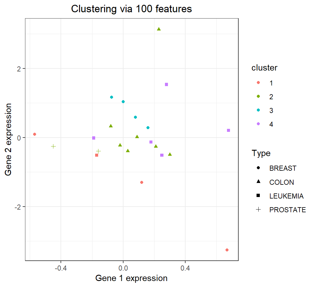
Clustering: comparison with truth

Plot the expressions of the 1st and 2nd genes in nci_a1 (to track observations), coloring via kmeans cluster membership and assigning shape via cancer type:

> nci_b = data.frame(nci_b)
> nci_b$Type = factor(colnames(nci_a1))
> nci_b$cluster = factor(clIdx$cluster)
> library(ggplot2)
> p3 = ggplot(nci_b,aes(X1,X2))+xlab("Gene 1 expression")+
+   ylab("Gene 2 expression")+theme_bw()+
+   geom_point(aes(shape=Type,color=cluster),na.rm = T)+
+   theme(legend.position="right")+
+   ggtitle("Clustering via 100 features")+
+   theme(plot.title = element_text(hjust = 0.5))

• legend.position="right": legend on right side of plot

Clustering: comparison with truth

\(22\) observations of nci_a1 in 4 clusters:

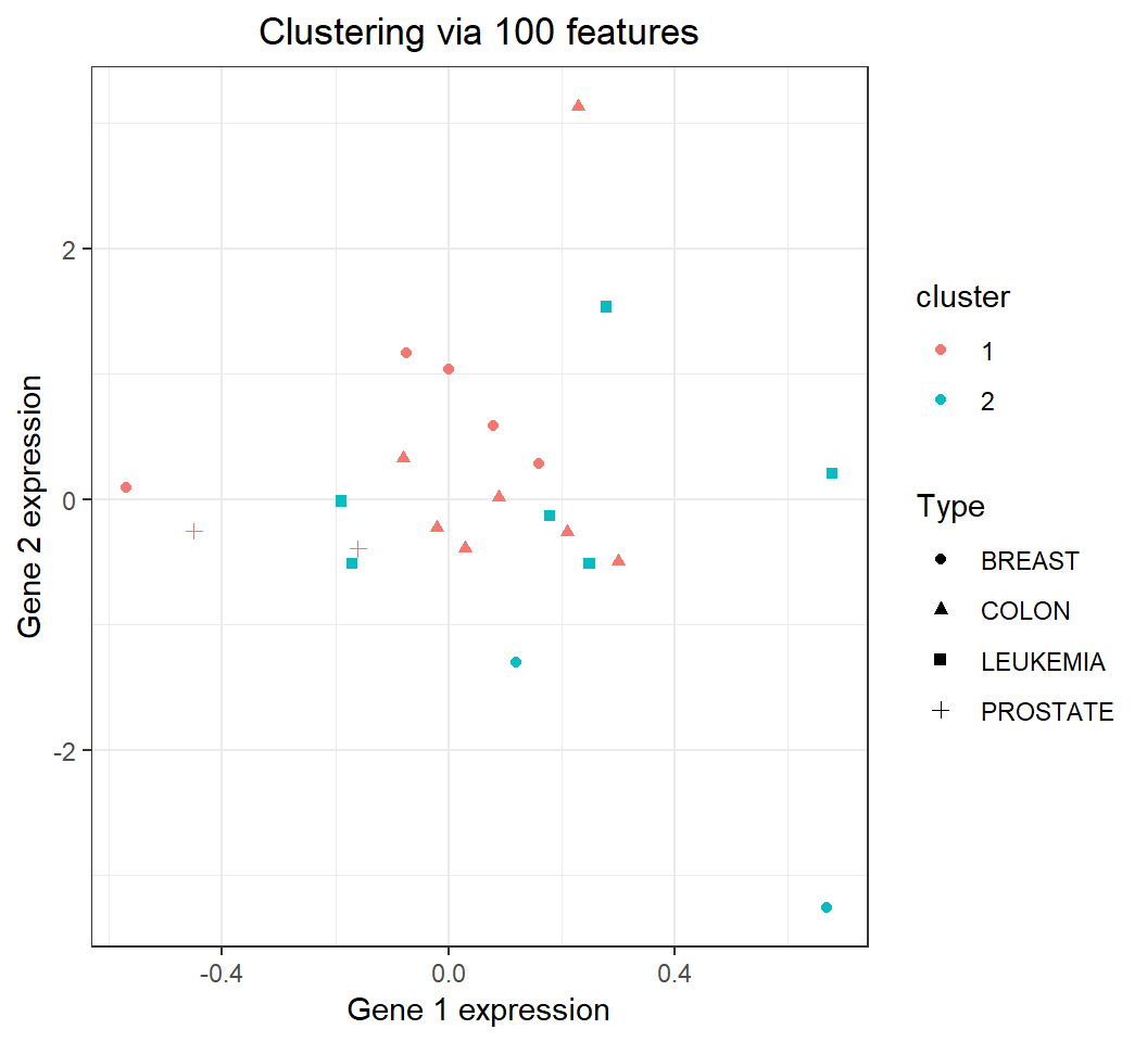
Clustering “nci_a1”: K=2

Split \(22\) observations in nci_a1 into \(2\) clusters (using the same settings for other arguments of kmeans):

> nci_b1 = t(nci_a1)
> set.seed(123)
> clIdxB = kmeans(nci_b1, 2, iter.max=30, nstart=20)
> clIdxB$cluster
  BREAST   BREAST   BREAST   BREAST   BREAST   BREAST   BREAST 
       1        1        1        2        2        1        1 
   COLON    COLON    COLON    COLON    COLON    COLON    COLON 
       1        1        1        1        1        1        1 
PROSTATE PROSTATE LEUKEMIA LEUKEMIA LEUKEMIA LEUKEMIA LEUKEMIA 
       1        1        2        2        2        2        2 
LEUKEMIA 
       2 

Clustering: comparison with truth

22 observations in nci_a1 (tracked by expressions of the 1st and 2nd genes) in 2 clusters:

Remarks

• In general, if there are \(K_0\) clusters in data, then \(K\)-means clustering with \(K < K_0\) will never be able to provide excellent clustering with respect to the underlying clusters.

• Clustering performance for the subset nci_a1 (with 100 features) may improve or become worse by including more features (i.e., more genes)

Clustering via more features

• Extract from nci observations for \(1000\) randomly sampled genes and for 4 cancer types “BREAST”, “COLON”, “PROSTATE”, and “LEUKEMIA”
• Save extracted observations as object nci_a2
• Split observations in nci_a2 into 4 clusters by kmeans based on 1000 features

Note: R codes to obtain nci_a2 are almost identical to those for obtaining nci_a1, except a change to sample as:

sample(1:dim(nci)[1], size=1000, replace = FALSE)

Visual comparison

\(22\) observations in 4 clusters:

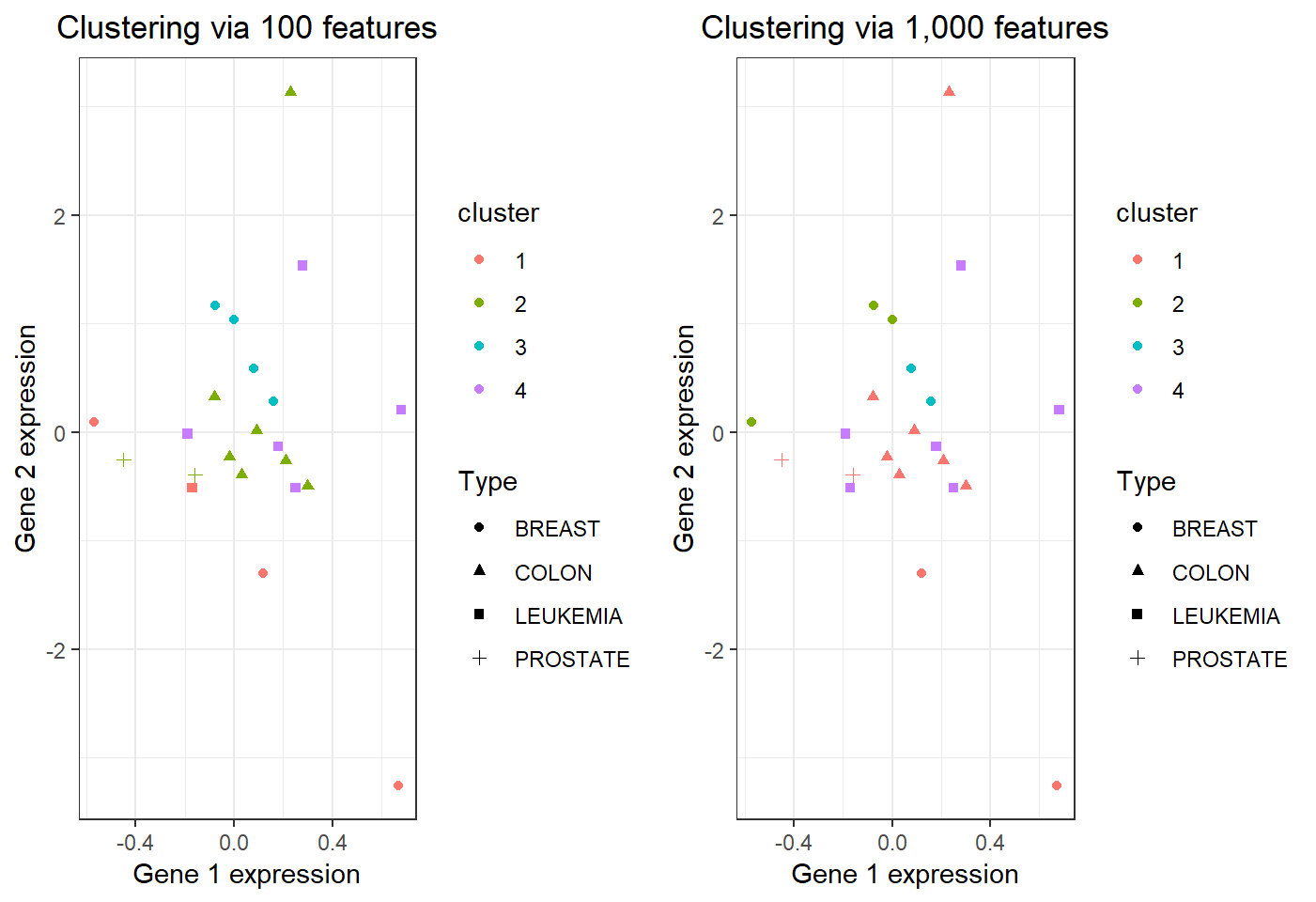
Summary of comparison

With more features,

• clustering observations for “PROSTATE” or “COLON” cancer does not improve or become worse
• clustering observations for “BREAST” cancer becomes worse as they are split into 3 clusters (from being split 2 clusters with less features)
• clustering observations for “LEUKEMIA” cancer improves since they are put into 1 cluster

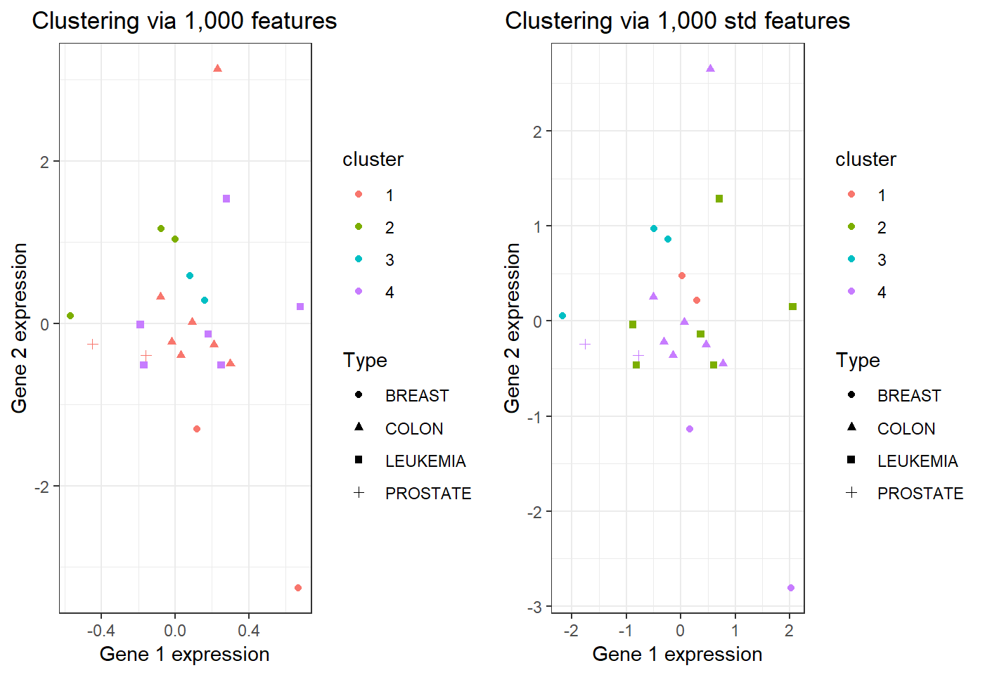
Standardization and clustering

Center and scale nci_a2 as standardization:

> nci_d = scale(t(nci_a2),center = TRUE, scale = TRUE)
> nci_d = data.frame(nci_d)
> set.seed(123)
> clIdxC=kmeans(nci_d,4,iter.max=30,nstart=20)
> nci_d$Type = factor(colnames(nci_a2))
> nci_d$cluster = factor(clIdxC$cluster)
> library(ggplot2)
> p6 = ggplot(nci_d,aes(X1,X2))+xlab("Gene 1 expression")+
+   ylab("Gene 2 expression")+theme_bw()+
+   geom_point(aes(shape=Type,color=cluster),na.rm = T)+
+   theme(legend.position="right")+
+  ggtitle("Clustering via 1,000 std features")+
+   theme(plot.title = element_text(hjust = 0.5))

Note: scale(x,center=TRUE, scale=TRUE) sets each column of x to have sample mean 0 and sample standard deviation 1.

Visual comparison

\(22\) observations in 4 clusters:

Estimate number of clusters

Estimate the true number of clusters for nci_a1 (that has 100 features and 4 underlying clusters) by gap statistic:

> library(cluster) 
> gap <- clusGap(t(nci_a1), kmeans, K.max=10, B=200,
+                iter.max=30, nstart=20)
> k <- maxSE(gap$Tab[, "gap"], gap$Tab[, "SE.sim"], 
+            method="Tibs2001SEmax")
> k
[1] 1
> # k is the estimated number of clusters

Note: correct estimate given by gap statistic.

Note: clusGap(t(nci_a) in lecture video should be clusGap(t(nci_a1).

Summary

• This supplementary verifies identity (10.12) of the Text
• This supplementary is not a required course material

The loss function

Recall the cluster assignment \(C: i \mapsto k\), i.e., \(C\) that assigns the \(i\)th observation \(\boldsymbol{x}_i\) to Cluster \(k\). For the dissimilarity \(D_{ii^{\prime}} =\Vert \boldsymbol{x}_i - \boldsymbol{x}_{i^{\prime}} \Vert^2 = d^2(\boldsymbol{x}_i,\boldsymbol{x}_{i^{\prime}})\), a “loss function” is \[ \begin{aligned} W(C) & = \sum_{k=1}^K \frac{1}{N_k}\sum_{C(i)=k} \sum_{C(i^{\prime})=k} D_{ii^{\prime}} \\ & = \sum_{k=1}^K \frac{1}{N_k} \sum_{C(i)=k} \sum_{C(i^{\prime})=k} \Vert \boldsymbol{x}_i - \boldsymbol{x}_{i^{\prime}} \Vert^2 \end{aligned} \]

The loss function \(W(C)\) for the assignment \(C\) measures the quality of clustering in terms of the dissimilarity \(D\).

K-means minimizing the loss

Recall \[ W(C) = \sum_{k=1}^K \frac{1}{N_k} \sum_{C(i)=k} \sum_{C(i^{\prime})=k} \Vert \boldsymbol{x}_i - \boldsymbol{x}_{i^{\prime}} \Vert^2 \]

K-means is equivalent to \[ C_{\ast}= \underset{C \in \mathcal{C}}{\operatorname{argmin}} W(C), \] where \(\operatorname{argmin}\) refers to “an argument that minimizes the objective”.

The minimizer \(C_{\ast}\), i.e., the optimal clustering assignment, is found over the set of all assignments \(\mathcal{C}\) of the \(N\) observations into \(K\) clusters.

Minimization of the loss

It can be verified that \[ \begin{aligned} & \sum_{k=1}^K \frac{1}{N_k} \sum_{C(i)=k} \sum_{C(i^{\prime})=k} \Vert \boldsymbol{x}_i - \boldsymbol{x}_{i^{\prime}} \Vert^2 \\ & = 2\sum_{k=1}^K \sum_{C(i)=k} \Vert \boldsymbol{x}_i - \bar{\boldsymbol{x}}_{k} \Vert^2, \end{aligned} \] where \[ \bar{\boldsymbol{x}}_{k} = \frac{1}{N_k} \sum_{i \in G_k} \boldsymbol{x}_i, \] \(G_k \subseteq \{1,\ldots,N\}\) is the index set for cluster \(k\), and \(N_k\) is the number of observations in cluster \(k\)

Verificiation

\[ \begin{aligned} & \sum_{k=1}^K \frac{1}{N_k}\sum_{C(i)=k} \sum_{C(i^{\prime})=k} \Vert \boldsymbol{x}_i - \boldsymbol{x}_{i^{\prime}} \Vert^2 \\ & = \sum_{k=1}^K \frac{1}{N_k}\sum_{C(i)=k} \sum_{C(i^{\prime})=k} \left( \Vert \boldsymbol{x}_i - \bar{\boldsymbol{x}}_{k} \Vert^2 + \Vert \boldsymbol{x}_{i^{\prime}} - \bar{\boldsymbol{x}}_{k} \Vert^2 \right)\\ & -\sum_{k=1}^K \frac{1}{N_k}\sum_{C(i)=k} \sum_{C(i^{\prime})=k} \left(\boldsymbol{x}_i - \bar{\boldsymbol{x}}_{k} \right) \left(\boldsymbol{x}_{i^{\prime}} - \bar{\boldsymbol{x}}_{k} \right)^T\\ \end{aligned} \]

Verificiation (cont’d)

However, \[ \begin{aligned} &\sum_{C(i)=k} \sum_{C(i^{\prime})=k} \left(\boldsymbol{x}_i - \bar{\boldsymbol{x}}_{k} \right) \left(\boldsymbol{x}_{i^{\prime}} - \bar{\boldsymbol{x}}_{k} \right)^T \\ & = - \sum_{C(i)=k} \sum_{C(i^{\prime})=k} \left( \boldsymbol{x}_i \bar{\boldsymbol{x}}_{k}^T + \boldsymbol{x}_{i^{\prime}}\bar{\boldsymbol{x}}_{k}^T \right) \\ & + \sum_{C(i)=k} \sum_{C(i^{\prime})=k} \boldsymbol{x}_i \boldsymbol{x}_{i^{\prime}}^T + N_k^2 \bar{\boldsymbol{x}}_{k} \bar{\boldsymbol{x}}_{k}^T\\ & = - N_k^2 \bar{\boldsymbol{x}}_{k} \bar{\boldsymbol{x}}_{k}^T + \sum_{C(i)=k} \sum_{C(i^{\prime})=k} \boldsymbol{x}_i \boldsymbol{x}_{i^{\prime}}^T = 0\\ \end{aligned} \]

Verificiation (cont’d)

So, \[ \begin{aligned} & \sum_{k=1}^K \frac{1}{N_k}\sum_{C(i)=k} \sum_{C(i^{\prime})=k} \Vert \boldsymbol{x}_i - \boldsymbol{x}_{i^{\prime}} \Vert^2 \\ & = \sum_{k=1}^K \frac{1}{N_k}\sum_{C(i)=k} \sum_{C(i^{\prime})=k} \left( \Vert \boldsymbol{x}_i - \bar{\boldsymbol{x}}_{k} \Vert^2 + \Vert \boldsymbol{x}_{i^{\prime}} - \bar{\boldsymbol{x}}_{k} \Vert^2 \right)\\ & = 2\sum_{k=1}^K \sum_{C(i)=k} \Vert \boldsymbol{x}_i - \bar{\boldsymbol{x}}_{k} \Vert^2 \end{aligned} \]

Summary

• This supplementary is adapted from the Thick book
• This supplementary is not a required course material

Iterative algorithm for K-means

• For a given assignment \(C\), solve for the centroids \(\left\{m_k\right\}_{k=1}^K\) via \[ \min_{\left\{m_k\right\}_{k=1}^K} \sum_{k=1}^K \sum_{C(i)=k} \Vert \boldsymbol{x}_i - m_{k} \Vert^2 \]
• For a given \(\left\{m_k\right\}_{k=1}^K\), solve for cluster assignment \(C\) via \[ C(i) = \underset{1 \le k \le K}{\operatorname{argmin}} \Vert \boldsymbol{x}_i - m_{k} \Vert^2 \]
• Iterate the above two until the assignments do not change

Remark on the Algorithm

Given observations \(\boldsymbol{x}_i, i \in S\) and let \(\bar{\boldsymbol{x}}_{S} = |S|^{-1} \sum_{i=1}^{|S|} \boldsymbol{x}_i\), then \(\bar{\boldsymbol{x}}_{S}\) minimizes the sum of squared Euclidean norms:

\[ \bar{\boldsymbol{x}}_{S} = \underset{m}{\operatorname{argmin}} \sum_{i \in S} \Vert \boldsymbol{x}_i - m \Vert^2 \] So, the algorithm solves a slightly more general optimization problem than minimizing just \[ W(C)= 2 \sum_{k=1}^K \sum_{C(i)=k} \Vert \boldsymbol{x}_i - \bar{\boldsymbol{x}}_{k} \Vert^2, \]

License and session Information

License

> sessionInfo()
R version 3.5.0 (2018-04-23)
Platform: x86_64-w64-mingw32/x64 (64-bit)
Running under: Windows 10 x64 (build 19041)

Matrix products: default

locale:
[1] LC_COLLATE=English_United States.1252 
[2] LC_CTYPE=English_United States.1252   
[3] LC_MONETARY=English_United States.1252
[4] LC_NUMERIC=C                          
[5] LC_TIME=English_United States.1252    

attached base packages:
[1] stats     graphics  grDevices utils     datasets  methods  
[7] base     

other attached packages:
[1] gridExtra_2.3 ggplot2_3.1.0 knitr_1.21   

loaded via a namespace (and not attached):
 [1] Rcpp_1.0.3       rstudioapi_0.8   magrittr_1.5    
 [4] tidyselect_0.2.5 munsell_0.5.0    colorspace_1.3-2
 [7] R6_2.3.0         rlang_0.4.4      dplyr_0.8.4     
[10] stringr_1.3.1    plyr_1.8.4       tools_3.5.0     
[13] revealjs_0.9     grid_3.5.0       gtable_0.2.0    
[16] xfun_0.4         withr_2.1.2      htmltools_0.3.6 
[19] assertthat_0.2.0 yaml_2.2.0       lazyeval_0.2.1  
[22] digest_0.6.18    tibble_2.1.3     crayon_1.3.4    
[25] purrr_0.2.5      glue_1.3.0       evaluate_0.12   
[28] rmarkdown_1.11   labeling_0.3     stringi_1.2.4   
[31] compiler_3.5.0   pillar_1.3.1     scales_1.0.0    
[34] pkgconfig_2.0.2