Recap on K-means

To implement K-means clustering, a user needs to specify

• the number of clusters to obtain
• initial centers for clusters to start the optimization process

However, it is not easy to accurately estimate the true number of clusters in data

Overview on HC

Hierarchical clustering

• does not have the two disadvantages of K-means
• requires a measure of dissimilarity between (disjoint) groups (or clusters) of observations
• often produces hierarchical clusters, where each observation is a cluster at the finest level, clusters with increasing dissimilarities are nested, and all observations form one cluster at the coarsest level

However, users need to determine which level of hierarchy is sensible to obtain the eventual clusters

Two modes of HC

Two modes of hierarchical clustering

• “bottom-up” (or “agglomerative”): start with the finest level, merge two clusters with the smallest intergroup dissimilarity, and keep iterating until one cluster is obtained
• “top-down” (or “divisive”): start with the coarsest level, split the cluster into two groups with the largest intergroup dissimilarity, and keep iterating until each observation is a cluster

We will focus on “bottom-up”" (or “agglomerative”) HC

Illustration by simulated data

• 45 observations \(x_i,i=1,\ldots,45\)
• each observation \(x_i\) is 2-dimensional vector
• the 45 observations form 3 distinct classes

Note: distinct class labels will be indicated by distinct colors

Illustration by simulated data

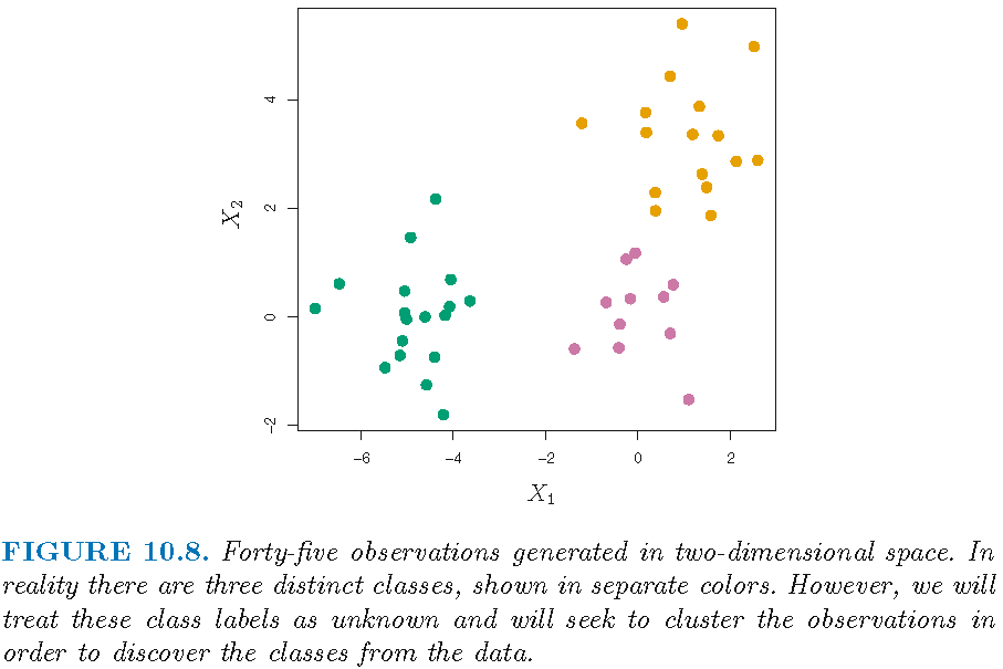
Illustration by simulated data

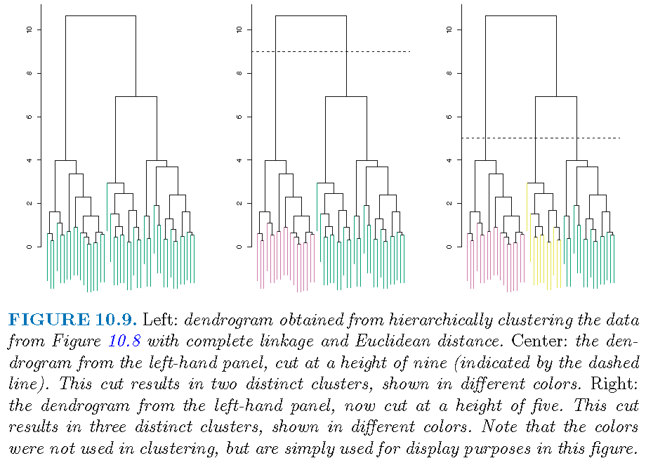
Suppose we do not know the class labels and perform hierarchical clustering by using

• Euclidean distance as the dissimilarity measure between each pair of observations
• complete linkage for disjoint groups that is based on Euclidean distance (to be discussed later)

We obtain a dendrogram that represents hierarchical clustering results as a tree-like structure

Illustration by simulated data

Understanding a dendrogram

A dendrogram is an upside-down tree with a height bar, where

• clusters at the bottom of the tree are leafs, where each leaf is an observation and a cluster
• as we move up the tree from the bottom, leafs begin to fuse into branches, and leafs and branches into branches
• the dissimilarity between two clusters indicates the height in the dendrogram at which these two clusters should be fused
• the larger the height is, the more dissimilar the branches or leafs are from each other at this height

Understanding a dendrogram

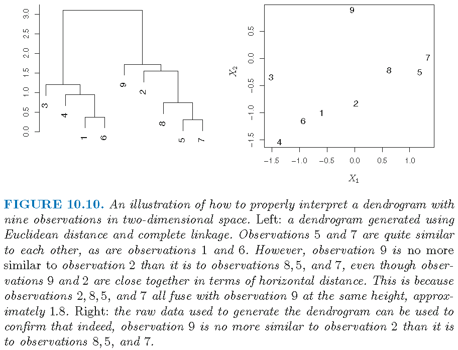
Understanding a dendrogram

When hierarchical clustering is represented by a dendrogram,

• the degree of similarity between two clusters is not determined by the horizontal distance between them on the dendrogram
• switching the left-right orientation of clusters at a given height that are subclusters of the same, immediate parent cluster does not change hierarchical clustering results

Caution on hierarchical clusters

• Hierarchical clustering often produces hierarchical clusters, where clusters obtained by cutting the dendrogram at a given height (i.e., clusters at a given height) are necessarily nested within the clusters obtained by cutting the dendrogram at any greater height (i.e., clusters at any greater height), when there is only one criterion that determines clusters or groups in the data

• However, hierarchical clustering will not necessarily be produced when sets of clusters are produced by different criteria

Caution on hierarchical clusters

Suppose we have observations from a group of people

• with a 50-50 split of males and females, giving the best two-group clustering that is obtained by gender
• evenly split among Americans, Japanese, and French, giving the best three-group clustering that is obtained by nationality

So, the two sets of groups are not nested, in the sense that the best 3-group clustering cannot be obtained splitting one group of the best 2-group clustering (since the group of people with the same nationality must contain people from both genders), and hence cannot be well represented by hierarchical clustering

Settings

• Assume there are \(p\) features \(x_j, j=1,\ldots,p\)
• Assume \(x_{ij},i=1,\ldots,n\) are \(n\) observations for the \(j\)th feature \(x_j\)
• Let \(\boldsymbol{x}_i = (x_{i1},\ldots,x_{ip}) \in \mathbb{R}^p\), i.e., \(\boldsymbol{x}_i\) is the \(i\)th observation for all \(p\) features

Using some dissimilarity measure, hierarchical clustering will split the \(n\) observations \(\boldsymbol{x}_i\) into sets of clusters at different dissimilarity levels (i.e., at different heights)

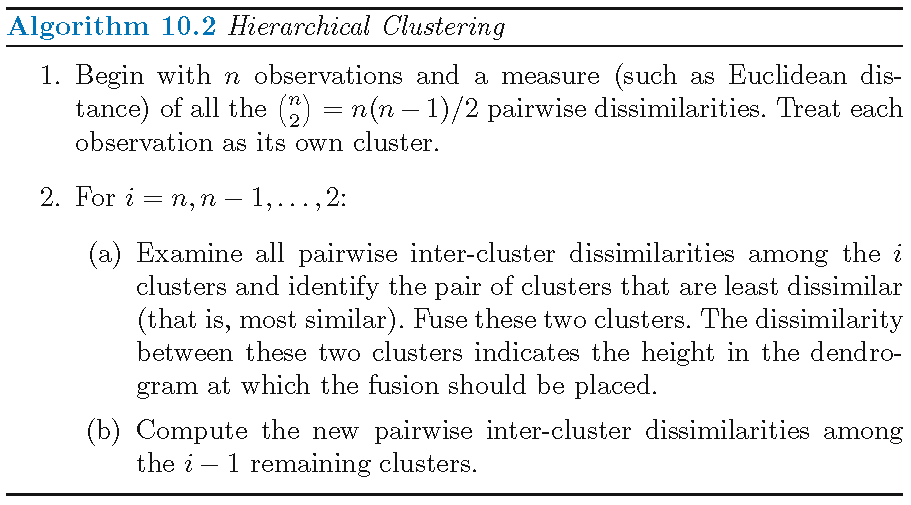
Agglomerative HC: algorithm

Dissimilarity meaures

The choice of a dissimilarity measure is crucial to hierarchical clustering, and there are many choices for this measure:

• Dissimilarity measure for each pair of observations (i.e., pairwise dissimilarity): Euclidean distance, the absolute value of sample correlation
• Dissimilarity measure for each pair of clusters (i.e., inter-cluster dissimilarity or linkage): complete linkage, single linkage, average linkage, centroid

Note: inter-cluster dissimilarity and pairwise dissimilarity should be compatible with each other in order to obtain hierarchical clustering

HC algorithm: illustration

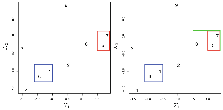
Agglomerative HC with Euclidean distance and complete linkage:

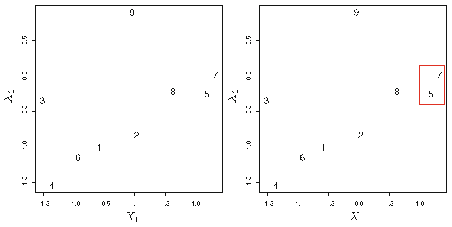
HC algorithm: illustration

Agglomerative HC with Euclidean distance and complete linkage:

Different linkages

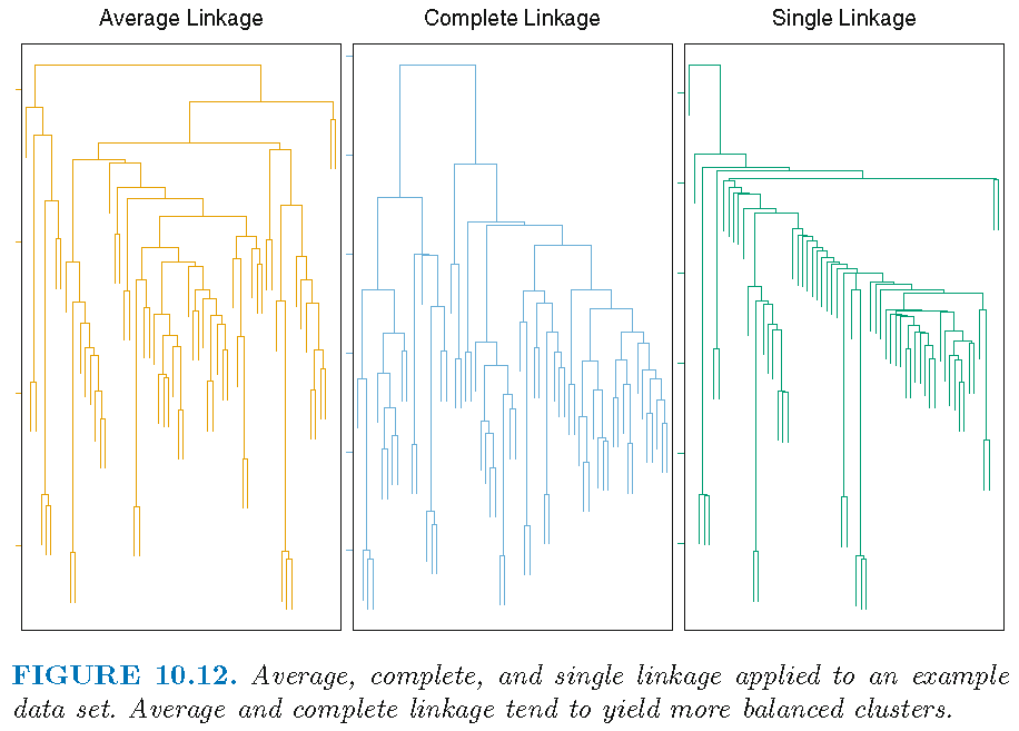
• Single linkage, i.e., minimal intercluster dissimilarity: compute all pairwise dissimilarities between the observations in cluster A and the observations in cluster B, and record the smallest of these dissimilarities. Single linkage can result in extended, trailing clusters in which single observations are fused one-at-a-time

• Centroid: dissimilarity between the centroid for cluster A and the centroid for cluster B. Centroid linkage may induce inversion in clustering, where two clusters are fused at a height below either of the individual clusters in the dendrogram

Different linkages

• Average linkage, i.e., mean intercluster dissimilarity: compute all pairwise dissimilarities between the observations in cluster A and the observations in cluster B, and record the average of these dissimilarities

• Complete linkage, i.e., maximal intercluster dissimilarity: compute all pairwise dissimilarities between the observations in cluster A and the observations in cluster B, and record the largest of these dissimilarities

Note: Average and complete linkages are generally preferred over single linkage, since they tend to yield more balanced dendrograms

Effects of linkage

Overview on practical issues

Some practical issues on hierarchical clustering:

• What pairwise dissimilarity measure to use?
• Is standardization needed for observations for each feature?
• Is cluster found by a clustering algorithm sensible?
• How to interpret clustering results?

Choice of dissimilarity measure

The choice of dissimilarity measure

• is very important since it has a strong effect on the resulting dendrogram
• should aim at capturing latent patterns in the data
• should be determined by the type of data being clustered and the scientific question at hand

Correlation-based distance

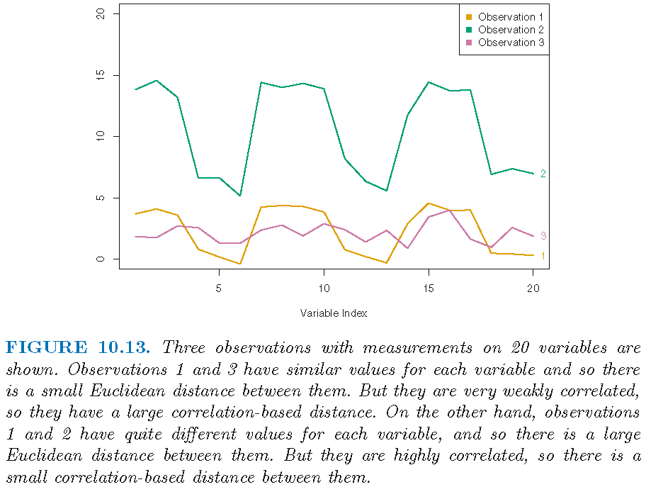
• Correlation-based distance considers 2 observations to be similar if their features are highly correlated, even though the observed values may be far apart in terms of Euclidean distance.
• There are various measures on correlation, such as the (Pearson’s) sample correlation, Spearman’s rank correlation, Kendall’s rank correlation
• Distance based on Pearson’s sample correlation is also based on standardized entries in each observation, due to how this correlation is computed. Hence, such a distance is not effected by the magnitude of observations in terms of Euclidean distance

Correlation-based distance

• \(3\) observations \(\boldsymbol{x}_i = (x_{i1},\ldots,x_{i,10}), i=1,2,3\) for \(10\) features
• let \(r_{kl}\) be Pearson sample correlation between the entries of \(\boldsymbol{x}_k\) and the entries of \(\boldsymbol{x}_l\), i.e., \[ r_{kl} = \frac{1}{p-1}\sum_{j=1}^p \frac{(x_{kj}-\bar{x}_k)}{s_k}\frac{(x_{lj}-\bar{x}_l)}{s_l}, k \ne l \] with \(\bar{x}_i = p^{-1}\sum_{j=1}^p x_{ij}\) and \[s_i^2 = (p-1)^{-1}\sum_{j=1}^p (x_{ij}-\bar{x}_i)^2\]
• if \(\vert r_{12} \vert > \vert r_{13} \vert\), then \(\boldsymbol{x}_1\) is more similar to \(\boldsymbol{x}_2\) than it is to \(\boldsymbol{x}_3\)

Correlation-based distance

Choice of dissimilarity measure

• Consider an online retailer interested in clustering shoppers based on their past shopping histories. The goal is to identify subgroups of similar shoppers, so that shoppers within each subgroup can be shown items and advertisements that are particularly likely to interest them.

• Suppose the data takes the form of a matrix where the rows are the shoppers and the columns are the items available for purchase; the elements of the data matrix indicate the number of times a given shopper has purchased a given item (i.e. a 0 if the shopper has never purchased this item, a 1 if the shopper has purchased it once, etc.)

Choice of dissimilarity measure

What type of dissimilarity measure should be used to cluster the shoppers?

• If Euclidean distance is used, then shoppers who have bought very few items overall (i.e. infrequent users of the online shopping site) will be clustered together. This may not be desirable.

• If correlation-based distance is used, then shoppers with similar preferences (e.g. shoppers who have bought items A and B but never items C or D) will be clustered together, even if some shoppers with these preferences are higher-volume shoppers than others.

Standardization of observations

• Consider an online retailer interested in clustering shoppers based on their past shopping histories. The goal is to identify subgroups of similar shoppers, so that shoppers within each subgroup can be shown items and advertisements that are particularly likely to interest them.

• Suppose the data takes the form of a matrix where the rows are the shoppers and the columns are the items available for purchase; the elements of the data matrix indicate the number of times a given shopper has purchased a given item (i.e. a 0 if the shopper has never purchased this item, a 1 if the shopper has purchased it once, etc.)

Standardization of observations

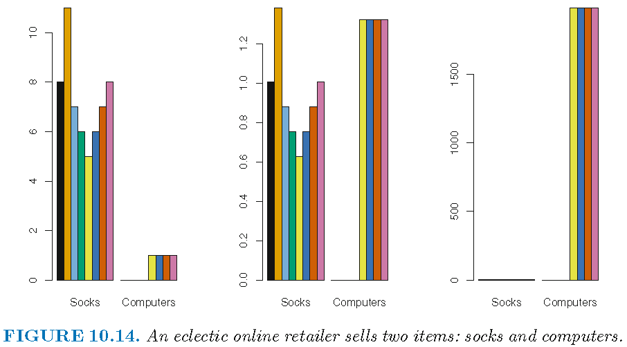
• If we choose a dissimilarity measure that is easily affected the magnitudes of observations, then high-frequency purchases like socks tend to have a much larger effect on the inter-shopper dissimilarities, and hence on the clustering ultimately obtained, than rare purchases like computers. This may not be desirable.

• If the variables are scaled to have standard deviation one before the inter-observation dissimilarities are computed, then each variable will in effect be given equal importance in the hierarchical clustering performed.

Standardization of observations

Left: raw data on purchase frequency; Center: scaled data on purchase frequency; Right: raw data on purchase expense

Standardization of observations

• We might also want to scale the variables to have standard deviation one if they are measured on different scales; otherwise, the choice of units (e.g. centimeters versus kilometers) for a particular variable will greatly affect the dissimilarity measure obtained.

• Whether or not it is a good decision to scale the variables before computing the dissimilarity measure depends on the application at hand.

• The issue of whether or not to scale the variables before performing clustering applies to K-means clustering as well.

Validation of obtained clusters

• Clusters are always formed when clustering is performed. But do the clusters that have been found represent true subgroups in the data, or are they simply a result of clustering the noise?
• For instance, if we were to obtain an independent set of observations, then would those observations also display the same set of clusters? This is a hard question to answer.
• There exist a number of techniques for assigning a p-value to a cluster in order to assess whether there is more evidence for the cluster than one would expect due to chance. However, there has been no consensus on a single best approach.

Robustness on clustering

Suppose that most of the observations truly belong to a small number of (unknown) subgroups, and a small subset of the observations are quite different from each other and from all other observations.

• Since both K-means and hierarchical clustering will assign each observation to a cluster, the clusters found may be heavily distorted due to the presence of outliers that do not belong to any cluster.

• Mixture models are an attractive approach for accommodating the presence of such outliers.

Robustness on clustering

Suppose that we cluster \(n\) observations, and then cluster the observations again after removing a subset of the \(n\) observations at random.

• We would hope that the two sets of clusters obtained would be quite similar. But often this is not the case!

• Clustering methods generally are not very robust to perturbations to the data.

Recommendations on clustering

• Perform clustering with different choices of standardization, dissimilarity measures, and linkages, and look at the full set of results in order to see what patterns consistently emerge.

• Clustering subsets of the data in order to get a sense of the robustness of the clusters obtained.

• Clustering results should not be taken as the absolute truth about a data set. Rather, they should constitute a starting point for the development of a scientific hypothesis and further study, preferably on an independent data set.

R software needed

R commands and libraries needed:

• R built-in command dist or as.dist to compute pairwise dissimilarity
• R built-in command hclust applies to pairwise dissimilarities to implement HC
• R built-in command cutree applies to the output of hclust to obtain clusters
• R library ggdendro and command ggdendrogram{ggdendro} create dendrogram from the output of hclust

Workflow

Workflow for software implementation:

• obtain pairwise dissimilarities
• implement hierarchical clustering
• show dendrogram

Command: dist

dist computes and returns the distance matrix that is obtained by using the specified distance measure to compute the distances between the rows of a data matrix. Its basic syntax is

dist(x, method = "euclidean")

• x: a numeric matrix, data frame or “dist” object.
• method: the distance measure to be used. It must be one of “euclidean”, “maximum”, “manhattan”, “canberra”, “binary” or “minkowski”.

Command: as.dist

as.dist converts an arbitrary square symmetric matrix into a form that hlust recognizes as a distance matrix. It can be used to induce correlation-based distance. Its basic syntax is

as.dist(x, ...)

• x: a numeric matrix, data frame or “dist” object.

Command: hclust

hclust implements hierarchical cluster analysis on a set of dissimilarities using a specified linkage. Its basic syntax is

hclust(d, method = "complete")

• d: a dissimilarity structure as produced by dist
• method: the agglomeration method to be used. It can be “single”, “complete”, “average” or “centroid”

Command: hclust

When clustering \(n\) observations, hclust returns:

• height: a set of \(n-1\) real values that are called “clustering heights”. Each height is the value of the dissimilarity measure for the corresponding agglomeration.
• labels: labels for each of the objects being clustered.

Command: cutree

cutree cuts a tree, e.g., as resulting from hclust, into several groups either by specifying the desired number(s) of groups or the cut height(s). Its basic syntax is

cutree(tree, k = NULL, h = NULL)

• tree: a tree as produced by hclust.
• k: an integer scalar or vector with the desired number of groups.
• h: numeric scalar or vector with heights where the tree should be cut.

Command: ggdendrogram

ggdendrogram{ggdendro} creates a dendrogram using the output of hclust. Its basic syntax is

library(ggdendro)
ggdendrogram(data, leaf_labels = TRUE, rotate = FALSE)

• data: objects of class dendrogram, hclust or tree
• leaf_labels: if TRUE, shows leaf labels
• rotate: if TRUE, rotates plot by 90 degrees

Note: the command plot can be applied to hclust object to create dendrogram

License and session Information

License

> sessionInfo()
R version 3.5.0 (2018-04-23)
Platform: x86_64-w64-mingw32/x64 (64-bit)
Running under: Windows 10 x64 (build 19041)

Matrix products: default

locale:
[1] LC_COLLATE=English_United States.1252 
[2] LC_CTYPE=English_United States.1252   
[3] LC_MONETARY=English_United States.1252
[4] LC_NUMERIC=C                          
[5] LC_TIME=English_United States.1252    

attached base packages:
[1] stats     graphics  grDevices utils     datasets  methods  
[7] base     

other attached packages:
[1] knitr_1.21

loaded via a namespace (and not attached):
 [1] compiler_3.5.0  magrittr_1.5    tools_3.5.0    
 [4] htmltools_0.3.6 revealjs_0.9    yaml_2.2.0     
 [7] Rcpp_1.0.0      stringi_1.2.4   rmarkdown_1.11 
[10] stringr_1.3.1   xfun_0.4        digest_0.6.18  
[13] evaluate_0.12