HC software implementation: Example 1
Example 1: generate data
Randomly generate observations from 2 bivariate Gaussian distributions with identity covariance matrix, so that
- the first 10 observations have mean vector \((3,0)\)
- the rest 10 observations have mean vector \((0,-4)\)
Namely, the 20 observations form 2 distinct groups according to their mean vectors, and there are 2 features.
> set.seed(2)
> x=matrix(rnorm(20*2), ncol=2)
> x[1:10,1]=x[1:10,1]+3; x[11:20,2]=x[1:10,2]-4
- each column of
x contains observations for a feature; each row of x contains an observation for 2 features
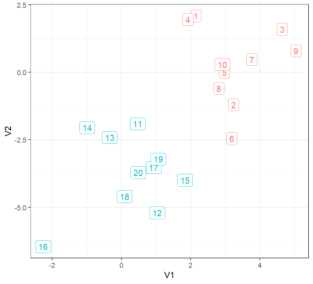
Example 1: visualize data
20 observations form 2 clusters:
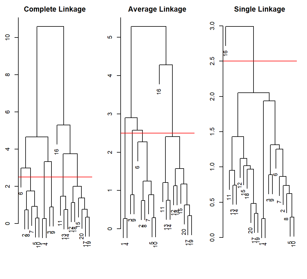
Example 1: clustering
Hierarchical clustering (with Euclidean distance as pairwise dissimilarity):
> hc.complete=hclust(dist(x), method="complete")
> hc.average=hclust(dist(x), method="average")
> hc.single=hclust(dist(x), method="single")
> par(mfrow=c(1,3))
> plot(hc.complete,main="Complete Linkage",xlab="",sub="",cex=.9)
> abline(h=2.5, col="red")
> plot(hc.average, main="Average Linkage",xlab="",sub="",cex=.9)
> abline(h=2.5, col="red")
> plot(hc.single, main="Single Linkage",xlab="",sub="",cex=.9)
> abline(h=2.5, col="red")
xlab="",sub="": set x-axis label and subtitle as the empty string; cex: ratio by which plotting text and symbols should be scaled relative to the default 1; note the abline at a given “height” h
Example 1: linkages in action
Good clustering results; differing clusters at the same height:
Example 1: heights and distances
height from “complete linkage” versus dist(x):
> hc.complete$height
 [1]  0.2702697  0.2906542  0.3423736  0.7377621  0.7428389
 [6]  0.7678718  0.8906271  0.9188777  1.1219922  1.3796578
[11]  1.4636674  1.7568482  1.9923715  2.9849541  3.3246916
[16]  3.7466658  4.6576892  5.2990990 10.5951990
> min(dist(x)) == min(hc.complete$height)
[1] TRUE
> max(hc.complete$height) == max(dist(x))
[1] TRUE
min(dist(x))=min(hc.complete$height), i.e., minimal pairwise dissimilarity equals to minimal heightmax(hc.complete$height): the value of linkage at which the last 2 clusters are merged
Example 1: heights and distances
height from “average linkage” versus dist(x):
> hc.average$height
 [1] 0.2702697 0.2906542 0.3423736 0.6260169 0.7377621
 [6] 0.7428389 0.8906271 0.8930763 1.1219922 1.1666896
[11] 1.2082378 1.2435332 1.5734885 2.2700984 2.4041542
[16] 2.5747045 2.8959725 4.2777927 5.2820763
> min(dist(x)) == min(hc.average$height)
[1] TRUE
> max(hc.average$height)
[1] 5.282076
> max(dist(x))
[1] 10.5952
min(dist(x))=min(hc.average$height), i.e., minimal pairwise dissimilarity equals to minimal heightmax(hc.complete$height): the value of linkage at which the last 2 clusters are merged
Example 1: heights and distances
Maximum of height is where the last 2 clusters are merged:
Example 1: cut dendrogram
Cut the dendrogram to obtain 2 clusters:
> cutree(hc.complete,2)
 [1] 1 1 1 1 1 1 1 1 1 1 2 2 2 2 2 2 2 2 2 2
> cutree(hc.average,2)
 [1] 1 1 1 1 1 1 1 1 1 1 2 2 2 2 2 2 2 2 2 2
> cutree(hc.single,2)
 [1] 1 1 1 1 1 1 1 1 1 1 1 1 1 1 1 2 1 1 1 1
- HC with single linkage assigns 1 observation as its own cluster
- HC with complete or average linkage splits the observations into their underlying groups
Example 1: height of cut
Cut tree to obtain 3 clusters and find the height of cut:
> hc.average$height
 [1] 0.2702697 0.2906542 0.3423736 0.6260169 0.7377621
 [6] 0.7428389 0.8906271 0.8930763 1.1219922 1.1666896
[11] 1.2082378 1.2435332 1.5734885 2.2700984 2.4041542
[16] 2.5747045 2.8959725 4.2777927 5.2820763
> clngrp = cutree(hc.average,k=3)
> clngrp
 [1] 1 1 1 1 1 1 1 1 1 1 2 2 2 2 2 3 2 2 2 2
> nh = length(hc.average$height)
> clhgt = cutree(hc.average,h=hc.average$height[nh-2])
> clhgt
 [1] 1 1 1 1 1 1 1 1 1 1 2 2 2 2 2 3 2 2 2 2
> all.equal(clngrp,clhgt)
[1] TRUE
cutree to obtain \(k\) groups is the same as cutree at the \(k\)th largest height
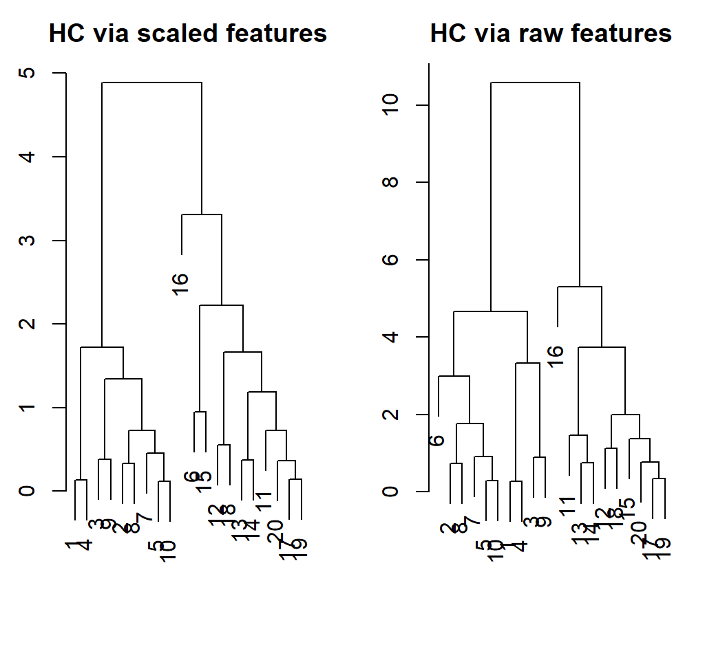
Example 1: scaling
HC with scaled features (i.e., each feature has standard deviation 1), Euclidean distance, and complete linkage:
> xsc=scale(x) # standardize each column (i.e., feature)
> par(mfrow=c(1,1),mar = c(7,4.5,0,1.4))
> plot(hclust(dist(xsc),method="complete"),xlab="",sub="",
+      main="",ylab="Height")
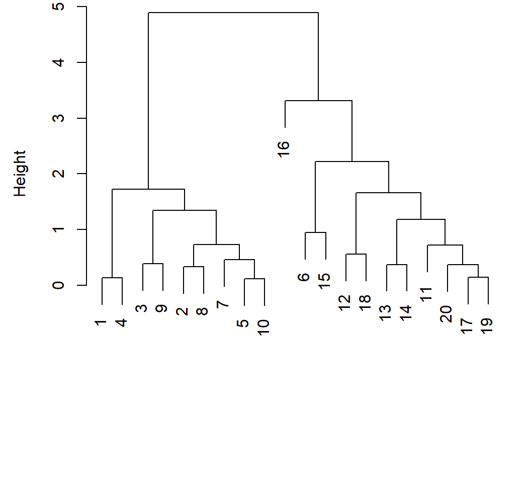
Example 1: scaling
With scaled features, obs. 6 and the last 10 obs. are put as a cluster; with original obs., we obtain the true groups
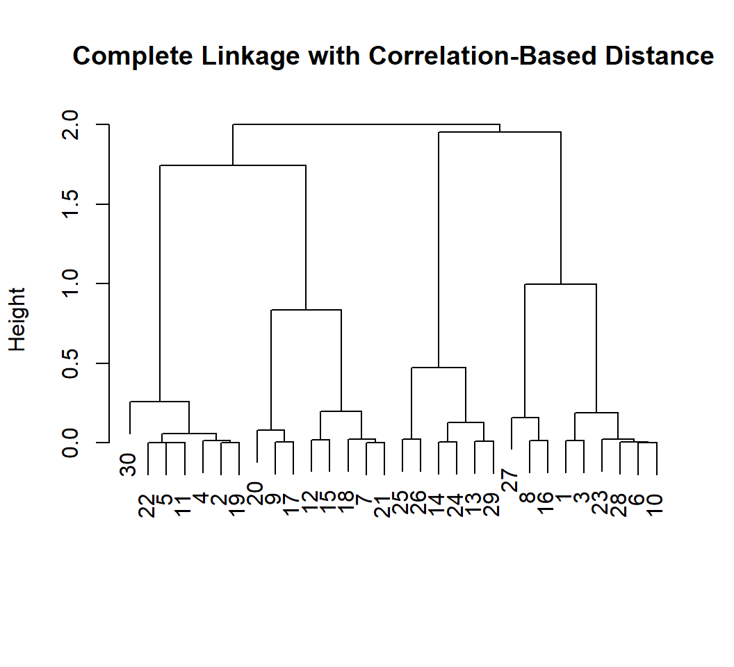
Example 1a: corr.-based distance
- Randomly generate 30 independent observations from a tri-variate Gaussian distribution with mean 0 and identity covariance matrix; put them in data matrix
x
> set.seed(1); x=matrix(rnorm(30*3), ncol=3)
> dd=as.dist(1-cor(t(x))) #corr.-based distance
x has 30 rows and 3 columns, i.e., there are 30 observations for 3 featurescor acts columnwise; we need to compute the correlation between each pair of observations, so we do cor(t(x))1-cor(t(x)) is a 30-by-30 symmetric matrix, each of whose entries is between 0 and 2
Example 1a: corr.-based distance
Truth is that the 30 observations form only 1 cluster in terms of what distributions they follow; but sample correlations are not zero for independent observations, leading to clusters:
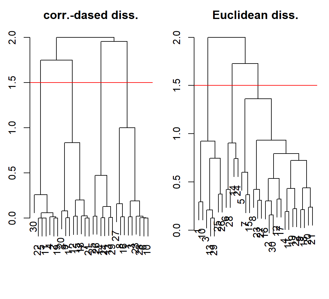
Example 1a: comparison
HC with complete linkage for dissimilarities on same scale:
HC software implementation: Example 2
Example 2: data
Human cancer microarray data:
- 6830 genes (i.e., 6830 features)
- 64 samples (i.e., 64 cancer cell lines, and each gene has 64 measurements)
- 14 different cancer types for the 64 samples (i.e., some samples are for one cancer type)
The data matrix has dimension \(64 \times 6830\); each row is an observation of all features
Example 2: data
> library(ISLR)
> nci.data=NCI60$data; nci.labs=NCI60$labs
> dim(nci.data)
[1]   64 6830
> nci.labs[1:4]
[1] "CNS"   "CNS"   "CNS"   "RENAL"
> table(nci.labs)
nci.labs
     BREAST         CNS       COLON K562A-repro K562B-repro
          7           5           7           1           1
   LEUKEMIA MCF7A-repro MCF7D-repro    MELANOMA       NSCLC
          6           1           1           8           9
    OVARIAN    PROSTATE       RENAL     UNKNOWN
          6           2           9           1
nci.data: gene expression data matrixnci.labs: cancer type for each sample; information on cancer types available at wiki-NCI60table(nci.labs) counts how many samples each cancer type has
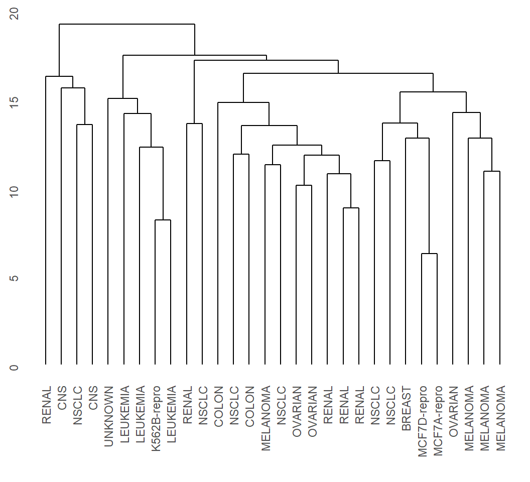
Example 2: scale and cluster
> sd.data=scale(nci.data) # standardize data
> # Euclidean norm as pairwise dissimiliarty
> data.dist=dist(sd.data)
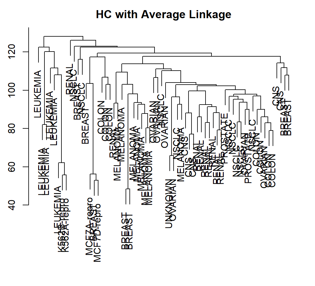
> plot(hclust(data.dist, method="average"), labels=nci.labs,
+ xlab="", sub="",ylab="", main="Average Linkage")
scale applies to each column of a matrix- each column of data matrix
nci.data contains observations for a feature (i.e., a variable)
- we need to standardize each variable (i.e., feature); so, we standardize observations for each feature (i.e., entries of each column) and use
scale(nci.data)
Example 2: visualize
Cell lines within a cancer type do tend to cluster together
Example 2: classification errors
> hc.al=hclust(dist(sd.data),method="average")
> hcal.clusters=cutree(hc.al,4)
> table(hcal.clusters,nci.labs)
             nci.labs
hcal.clusters BREAST CNS COLON K562A-repro K562B-repro
            1      7   5     7           0           0
            2      0   0     0           0           0
            3      0   0     0           1           1
            4      0   0     0           0           0
             nci.labs
hcal.clusters LEUKEMIA MCF7A-repro MCF7D-repro MELANOMA NSCLC
            1        0           1           1        8     8
            2        0           0           0        0     0
            3        6           0           0        0     0
            4        0           0           0        0     1
             nci.labs
hcal.clusters OVARIAN PROSTATE RENAL UNKNOWN
            1       6        2     8       1
            2       0        0     1       0
            3       0        0     0       0
            4       0        0     0       0
nci.labs: cancer type for each observation; the truth- all leukemia cell lines in cluster 3; all breast cancer cell lines in cluster 1
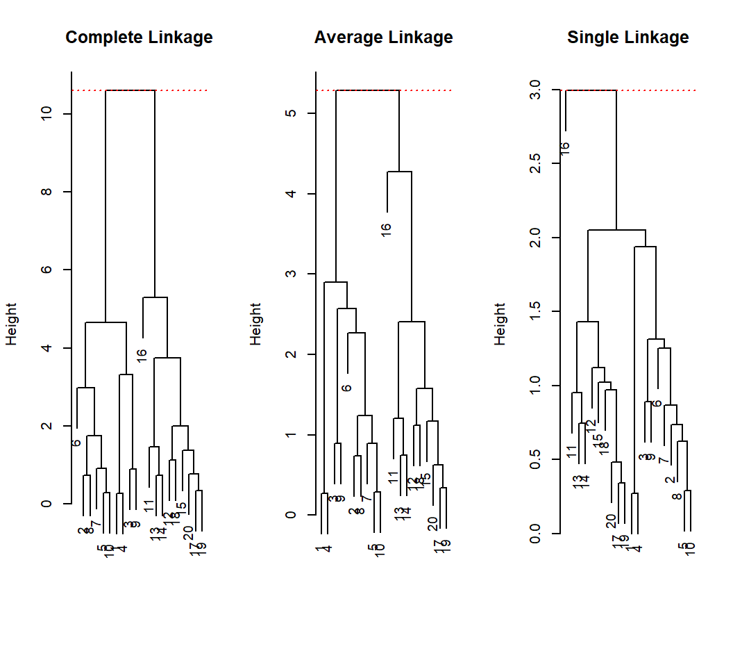
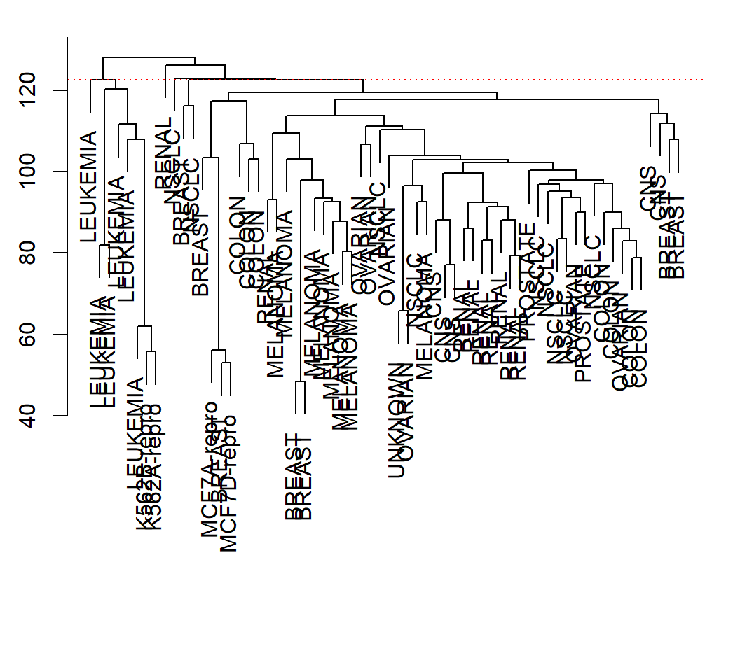
Example 2: height and clusters
> cutheight=hc.al$height[length(hc.al$height)-3]
> all.equal(cutree(hc.al,h=cutheight),cutree(hc.al,4))
[1] TRUE
> par(mfrow=c(1,1),mar = c(3.5,2.5,1.4,1.4))
> plot(hc.al, labels=nci.labs,xlab="", sub="",main="")
> abline(h=cutheight, col="red",lty="dotted")
HC software implementation: Example 3
Example 3: data
Human cancer microarray data:
- 6830 genes (i.e., 6830 features)
- 64 samples (i.e., 64 cancer cell lines)
- 14 different cancer types
The data matrix has dimension \(6830 \times 64\), each of whose columns is an observation for all features. We will randomly sample \(100\) genes and \(30\) samples, and use the measurements on these genes to cluster these samples.
Information on cancer types at wiki-NCI60
Example 3: subset of data
> library(ElemStatLearn) # library containing data
> data(nci); n = dim(nci)[2]; p = dim(nci)[1] #get dimensions
> set.seed(123)
> rSel = sample(1:p, size=100, replace = FALSE)
> cSel = sample(1:n, size=30, replace = FALSE)
> nci_a = nci[rSel,cSel]
> colnames(nci_a) = colnames(nci)[cSel]
- Caution: each column of
nci is an observation for all features; each row of nci contains observations for a feature
- take features (i.e., genes) from rows, and take samples (i.e., observations for features) from columns
- each column name is the cancer type for the observation
Example 3: subset of data
First few entries of data matrix nci_a:
     LEUKEMIA UNKNOWN   NSCLC MELANOMA OVARIAN
[1,]   0.6800  0.0800  0.2400  -0.2600  0.0200
[2,]   0.2075  0.1675 -1.4725   0.2775  0.1475
[3,]   0.1650  0.6950 -0.5750  -0.1050 -0.5250
- each column is an observation for all 100 features; each row contains 30 observations for a feature
- each column name is the cancer type for the observation
Example 3: obtain dissimilarity
> # Euclidean norm as pairwise dissimilarity
> # applied to scaled data
> dMat = dist(scale(t(nci_a)))
> length(dMat)
[1] 435
The command dist(scale(t(nci_a))):
- each row of
nci_a is a feature, leading to scale(t(nci_a)) since we standardize each feature
- each row of
scale(t(nci_a)) is an observation for all 100 standardized features, and then dist computes Euclidean distance between each pair of rows of scale(t(nci_a))
- 30 rows (i.e., observations) give 435 pairwise dissimilarities
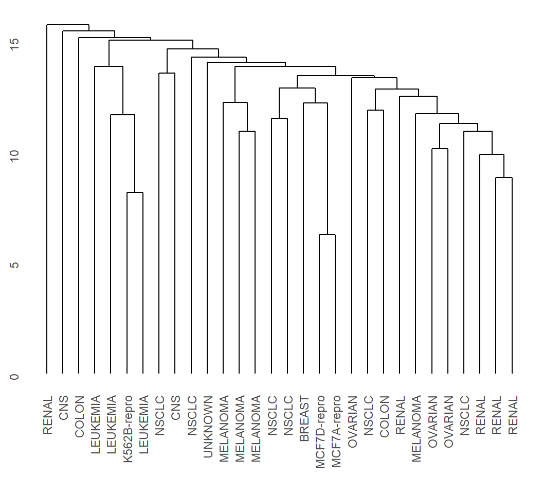
Example 3: average linkage
> EHC_al = hclust(dMat, method = "average")
> library(ggdendro)
> ggdendrogram(EHC_al, rotate = F)
Example 3: single linkage
> EHC_SL = hclust(dMat, method = "single")
> library(ggdendro)
> ggdendrogram(EHC_SL, rotate = F)
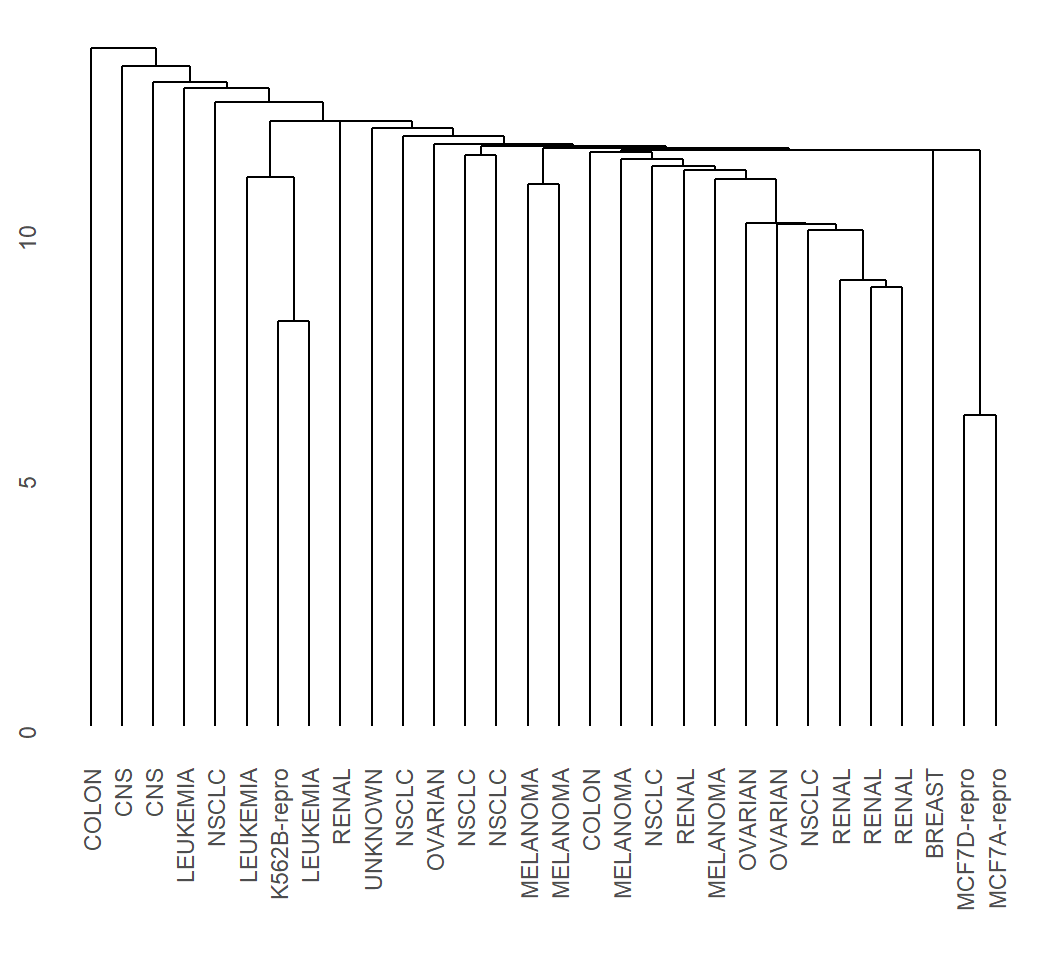
Example 3: complete linkage
> EHC_CL = hclust(dMat, method = "complete")
> library(ggdendro)
> ggdendrogram(EHC_CL, rotate = F)
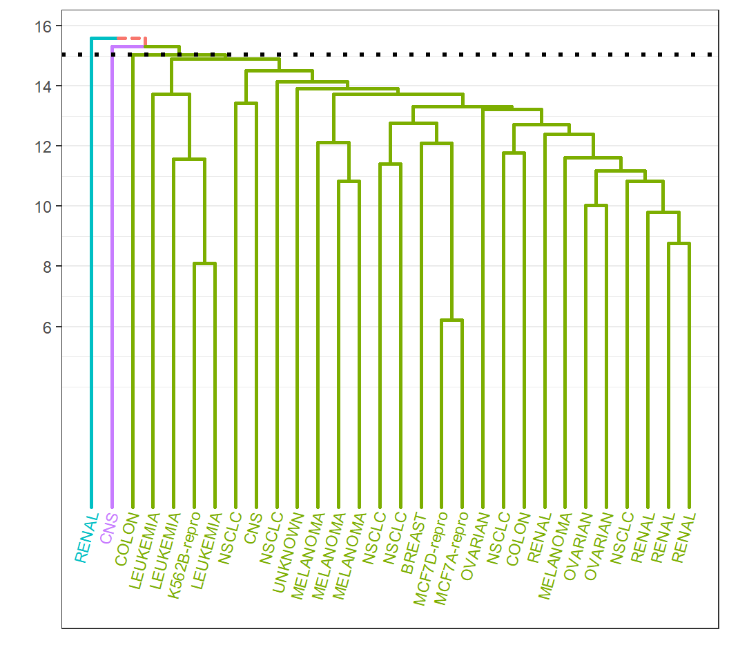
Example 3: customization
Customize dendrogram for EHC_al:
> library(ElemStatLearn); library(ggplot2)
> source("Plotggdendro.r")
> cutheight = EHC_al$height[length(EHC_al$height)-2]
> droplot = plot_ggdendro(dendro_data_k(EHC_al, 3),
+   direction = "tb",heightReferece=cutheight,expand.y = 0.2)
dendro_data_k(EHC_al,3): extract information on cutting the tree to obtain 3 groupscutheight: height at which 3 groups are obtained when cutting the treeplot_ggdendro: visualize tree at the hierarchy of 3 groups; plot_ggdendro contained in file “Plotggdendro.r”; credit at website
Example 3: customization
Leafs and branches for each group are colored: