Classification as a task

Classification is a very common and important task:

• check if an email is a spam or not
• detect if a tumor is benign or not
• determine if a product has defects or not

Classification is a more complicated task than clustering, since

• classification aims to assign the correct group or cluster label to each observation, whereas
• clustering only aims to assign a group or cluster label to each observation

Some methods of classification

Classification methods can be approximately categorized into “model-based” or “non-model based”.

• Some non-model based methods: k-nearest neighbor (kNN) classifiers, Support vector machines, Neural networks, Tree-based classifiers

• Some model-based methods: Bayes classifier, Discriminant analysis, Logistic regression

Overview

The Bayes classifier

• employs a Bayes model that uses prior, conditional, marginal, and posterior probabilities (or distributions)

• minimizes the expected 0-1 loss and is hence optimal (to be discussed later)

• serves as an unattainable gold standard against which to compare other classifiers (since for real data, we do not know the conditional distributions needed to implement this classifier)

Example data

• Flip a fair coin; if it lands on head, then generate an observation from the bivariate Gaussian distribution with mean vector \((3,0)\) and identity covariance matrix \(\mathbf{I}\), whereas if it lands on tail, then generate an observation from the bivariate Gaussian distribution with mean vector \((0,-4)\) and identity covariance matrix

• Repeat the above 10 times independently in order to obtain 10 observations

Namely, the 10 observations form 2 distinct groups according to their mean vectors, and there are 2 features.

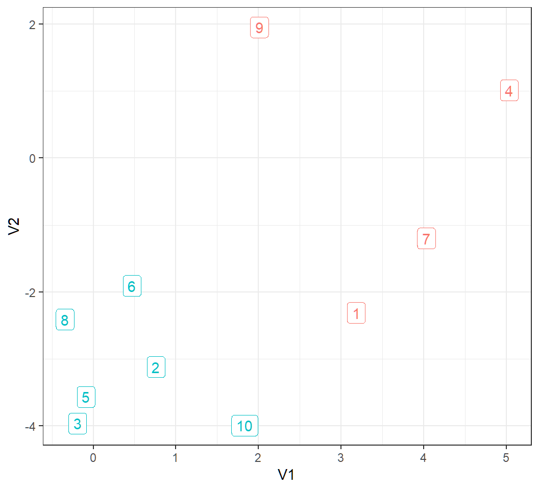
Visualize data

10 observations form 2 classes (observations 1, 4, 7 and 9 form a class, and the rest form another class):

Bayes two-group model

The data generating process can be formulated as follows:

• Let \(Y_i\) denote the class label (or group membership) of the observation \(x_i\) for \(i=1,\ldots,n\)

• There are 2 classes, i.e., \(Y_i =1\) for “Class 1” or \(Y_i=2\) for “Class 2”, such that, for some \(p \in (0,1)\) \[ \Pr(Y_i =1)=p, \quad \Pr(Y_i =2)=1-p \]

• If \(Y_i =1\), then \(x_i \sim \text{Gaussian}(\mu_1,\mathbf{\Sigma}_1)\), whereas if \(Y_i =2\), then \(x_i \sim \text{Gaussian}(\mu_2,\mathbf{\Sigma}_2)\)

Note: in the example, \(n=10\), \(p=0.5\), \(\mu_1=(3,0)\), \(\mu_2=(0,-4)\), \(\mathbf{\Sigma}_1=\mathbf{\Sigma}_2=\mathbf{I}\)

Prior and conditional distributions

• \(\Pr(Y_i =1)=p\) and \(\Pr(Y_i =2)=1-p\) are called the prior probabilities for class labels

• “If \(Y_i =1\), then \(x_i \sim \text{Gaussian}(\mu_1,\mathbf{\Sigma}_1)\)” means “the conditional density \(f_1\) of \(x_i\) given \(Y_i=1\) is the Gaussian density with mean vector \(\mu_1\) and covariance matrix \(\mathbf{\Sigma}_1\)”, and is written as \[ f_1(x | Y_i=1) \sim \text{Gaussian}(\mu_1,\mathbf{\Sigma}_1) \]

• Similarly, “if \(Y_i =2\), then \(x_i \sim \text{Gaussian}(\mu_2,\mathbf{\Sigma}_2)\)” means “the conditional density of \(x_i\) given \(Y_i=2\), denoted by \(f_2(x | Y_i=2)\) , is the Gaussian density with mean vector \(\mu_2\) and covariance matrix \(\mathbf{\Sigma}_2\)”

Marginal and posterior distr.

Given prior probabilities \[\Pr(Y_i =1)=p, \quad \Pr(Y_i =2)=1-p\] for the 2 classes and the conditional densities for \(x_i\) as \[f_j(x | Y_i=j) \sim \text{Gaussian}(\mu_j,\mathbf{\Sigma}_j),j=1,2\]

• the marginal density of \(x_i\) is \[ f(x) = f_1(x | Y_i=1) \Pr(Y_i =1) + f_2(x | Y_i=2) \Pr(Y_i =2) \]

• the posterior probability of \(x_i\) belonging to Class \(j\), i.e., the conditional probability of \(Y_i=j\) given \(x_i\), is \[ \Pr(Y_i=j|x_i) = \frac{f_j(x_i | Y_i=j) \Pr(Y_i =j)}{f(x_i)} \]

Compute posterior

For the example,

• \(\Pr(Y_i =1)=\Pr(Y_i =2)=0.5\)
• \(f_1(x | Y_i=1) \sim \text{Gaussian}(\mu_1=(3,0),\mathbf{I})\)
• \(f_2(x | Y_i=2) \sim \text{Gaussian}(\mu_2=(0,-4),\mathbf{I})\)

For \(x_1=(3.132420,-2.311069)\), we have

• \(f_1(x_1| Y_1=1)=0.01091\)
• \(f_2(x_1| Y_1=2)=0.00028\)
• \[ \begin{aligned} f(x_1) & = f_1(x_1| Y_1=1) \Pr(Y_1 =1) \\ & \quad + f_2(x_1 | Y_1=2) \Pr(Y_1 =2)\\ & = 0.5 \times 0.01091+0.5 \times 0.00028 = 0.00560 \end{aligned} \]

Compute posterior

The posteriors are:

• \[ \begin{aligned} \Pr(Y_1=1|x_1) & = \frac{f_1(x_1 | Y_1=1) \Pr(Y_1 =1)}{f(x_1)} \\ & = \frac{0.5 \times 0.01091}{0.00560}=0.9747 \end{aligned} \]

• \[ \begin{aligned} \Pr(Y_1=2|x_1) & = \frac{f_2(x_1 | Y_1=2) \Pr(Y_1 =2)}{f(x_1)} \\ & = \frac{0.5 \times 0.00028}{0.00560}=0.025259 \end{aligned} \]

Bayes classifier

• The Bayes classifier proposes to classify an observation to the class for which the corresponding posterior probability for the observation to belong to this class is the largest among all such posterior probabilities (that are computed for each class).

• Namely, \(x_i\) will be classified to Class \(\hat{j}\) if \[ \hat{j} = \operatorname*{argmax}\{j\in \{1,2\}: \Pr(Y_i=j|x_i)\} \]

Note: \(\operatorname*{argmax}\) returns the argument at which the maximum being sought is obtained

Bayes classifier

For the example,

• for observation \(x_1=(3.132420,-2.311069)\), we have \[\Pr(Y_1=1|x_1)=0.9747, \quad \Pr(Y_1=2|x_1)=0.025259\]

• Since \[\Pr(Y_1=1|x_1) > \Pr(Y_1=2|x_1),\] the Bayes classifier will classify \(x_1\) to Class \(1\)

• since there are 2 classes and \(\Pr(Y_1=1|x_1) + \Pr(Y_1=2|x_1)=1\), we must have \(\Pr(Y_1=1|x_1) > \Pr(Y_1=2|x_1)\) if and only if (“iff”) \(\Pr(Y_1=1|x_1) > 0.5\). So, the Bayes classifier will classify \(x_1\) to Class \(j\) if \(\Pr(Y_1=j|x_1) > 0.5\)

Example: posterior prob.

Posterior probability of each observation belonging to a class:

             PPCL1        PPCL2
 [1,] 9.747409e-01 2.525912e-02
 [2,] 1.046019e-03 9.989540e-01
 [3,] 2.095184e-06 9.999979e-01
 [4,] 1.000000e+00 1.683903e-10
 [5,] 1.384877e-05 9.999862e-01
 [6,] 5.296168e-02 9.470383e-01
 [7,] 9.999762e-01 2.380586e-05
 [8,] 6.620328e-04 9.993380e-01
 [9,] 1.000000e+00 3.390852e-08
[10,] 7.972362e-04 9.992028e-01

• column 1 contains such probabilities for Class 1
• column 2 contains such probabilities for Class 2

Bayes classifier

True class labels (TrueClass) and labels (EstClass) obtained by the Bayes classifier:

          PPCL1        PPCL2 TrueClass EstClass
1  9.747409e-01 2.525912e-02         1        1
2  1.046019e-03 9.989540e-01         2        2
3  2.095184e-06 9.999979e-01         2        2
4  1.000000e+00 1.683903e-10         1        1
5  1.384877e-05 9.999862e-01         2        2
6  5.296168e-02 9.470383e-01         2        2
7  9.999762e-01 2.380586e-05         1        1
8  6.620328e-04 9.993380e-01         2        2
9  1.000000e+00 3.390852e-08         1        1
10 7.972362e-04 9.992028e-01         2        2

Classification errors are zero:

   
    1 2
  1 4 0
  2 0 6

Remarks

To implement the Bayes classifier, we need to be able to obtain the marginal and posterior probabilities.

• In the example, we know the prior and conditional probabilities and are able to implement the Bayes classifier; further, since the observations are relatively well separated, the Bayes classifier has zero classification errors
• In practice, the prior and conditional probabilities need to be estimated, and so are the the marginal and posterior probabilities, leading to some difficulty in implementing the Bayes classifier (especially when the number of observations is much smaller than the number of features)

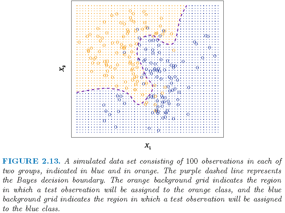
Bayesian decision boundary

Classification task

• Assume there are \(p\) features, and let \(x_{i}\), \(i=1,\ldots,N\) be the \(i\)th observation for these features

• Let \(G_{i}\) be the class label for \(x_{i}\) for each \(i=1,\ldots,N\)

• The \(N\) observations \(x_i\) form 2 distinct classes, i.e., \(G_{i}\in \mathcal{G}=\{1,2\}\) for all \(i\), and \(G_{i}\)’s are known; here \(\mathcal{G}\) is the set of distinct class labels

• The task: given a new observation \(x\) (from \(X\)) for the \(p\) features, estimate its class label \(G\), i.e., classify \(x\) into one of the 2 classes

Probabilistic formulation

• The observations on the features, i.e., \(x_i\)’s, are often regarded as a sample from a random vector \(X\)

• In Bayesian statistics, the class labels, i.e., \(G_i\)’s, are regarded as a sample from a random variable \(G\), to capture the postulation that for each observation \(x'\) from \(X\), its class label \(G'\) is random

• The performance of a classifier is measured by how well it classifies new observations on avarage by accounting for the randomness of \(X\) and \(G\) when new observations are obtained

The 0-1 loss

The “0-1 loss” as a measure on classification performance in a two-class classification task:

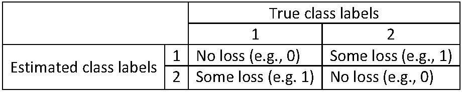
The 0-1 loss

• Let \(\hat{G}(x)\) be the estimated class label for an observation \(x\) from \(X\), i.e., \(\hat{G}(x)=1\) or \(2\)

• For \(k,l \in \{1,2\}\), the 0-1 loss \(L\) is defined as: \[L(k,l)=0 \text{ if } k=l \text{ and } L(k,l) =1 \text{ if } k \ne l \]

• Namely, let \(G(x)\) be the true class label for \(x\), then \(L(G(x),\hat{G}(x))=0\) when \(G(x)=\hat{G}(x)\) but \(L(G(x),\hat{G}(x))=1\) when \(G(x) \ne \hat{G}(x)\)

Namely, the loss \(L\) is \(0\) if and only if an observation is correctly classified; otherwise \(L\) is \(1\)

The expected 0-1 loss

• Let \(G(X)\) denote the true class label of \(X\). For each \(k \in \{1,2\}\), let \(\mathcal{G}_{k}=\left\{G(x):G(x)=k\right\}\) when \(X=x\); namely, \(\mathcal{G}_{k}\) is the set of class labels for Class \(k\) only

• Then the expected 0-1 loss is \[ \begin{aligned} \rho & =E(L[G(X),\hat{G}(X)]) \\ & = E_{X}\left( \sum_{k=1}^{2}L[\mathcal{G}_{k},\hat {G}(X)]\Pr(\mathcal{G}_{k}|X)\right), \end{aligned} \] where \(E_{X}\) denotes expectation with respect to the distribution of \(X\)

• Note: the expression for \(\rho\) holds for any loss \(L\)

The minimizer

• To minimize the expected 0-1 loss \[ \rho=E_{X}\left( \sum_{k=1}^{2}L[\mathcal{G}_{k},\hat{G}(X)]\Pr (\mathcal{G}_{k}|X)\right), \] we can minimize, for each value \(x\) of \(X\), the conditional loss \[ \rho(x; \hat{G}) = \sum_{k=1}^{2}L[\mathcal{G}_{k},\hat{G}(x)]\Pr (\mathcal{G}_{k}|x) \] for all possible classifiers \(\hat{G}\)
• \(\rho(x; \hat{G})\) has 2 summands. When \(L\) is the 0-1 loss, exactly one among \(L[\mathcal{G}_{1},\hat{G}(x)]\) and \(L[\mathcal{G}_{2},\hat{G}(x)]\) is \(0\), since \(\hat{G}(x)\) is either \(1\) or \(2\)

The minimizer

Recall \(\rho(x; \hat{G}) = \sum_{k=1}^{2}L[\mathcal{G}_{k},\hat{G}(x)]\Pr(\mathcal{G}_{k}|x)\)

• Let \(q_k(x)=\Pr(\mathcal{G}_{k}|x)\) for \(k \in \{1,2\}\) and set \[q(x)=\max\{q_1(x), q_2(x)\}\]

• If \(q(x)=q_1(x)\) and we set \(\hat{G}(x)=1\), then \[ L[\mathcal{G}_{1},\hat{G}(x)]=0, \quad L[\mathcal{G}_{2},\hat{G}(x)]=1 \] \(\rho(x; \hat{G}) = 0 \times q_1(x) + 1 \times q_2(x) = q_2(x)=\min\{q_1(x),q_2(x)\}\)

• Similarly, if \(q(x)=q_2(x)\) and we set \(\hat{G}(x)=2\), then \(\rho(x; \hat{G}) = 1 \times q_1(x) + 0 \times q_2(x) = q_1(x)=\min\{q_1(x),q_2(x)\}\)

The minimizer

• Since \(q_k(x)=\Pr(\mathcal{G}_{k}|x)\) and \(q_1(x)+q_2(x)=1\), in either case discussed previously, we must have \[ \begin{aligned} \rho(x; \hat{G}) & = \min\{\Pr(\mathcal{G}_{1}|x), \Pr(\mathcal{G}_{2}|x)\}\\ & = 1 - \max\{\Pr(\mathcal{G}_{1}|x), \Pr(\mathcal{G}_{2}|x)\} \end{aligned} \] when the classifier \(\hat{G}\) assigns an observation \(x\) from \(X\) to Class \(j\), where \[\Pr(\mathcal{G}_{j}|x)=\max\{\Pr(\mathcal{G}_{k}|x): k=1,2\}\]

• Thus, \(\rho(x; \hat{G})\) is minimized by the classifier given above, i.e., \[ \hat{G}(x) = \operatorname*{argmax} \{ g\in \{1,2\} : \Pr\left(g|X=x\right) \} \]

The Bayes classifier is optimal

• The the expected 0-1 loss \[ \rho =E(L[G(X),\hat{G}(X)]) \] is minimized by the classifier \[ \hat{G}(x) = \operatorname*{argmax} \{ g\in \{1,2\} : \Pr\left(g|X=x\right) \} \]

• The optimal classifier \(\hat{G}\) with \(x \to \hat{G}(x) \in \{1,2\}\) that is given above is called the Bayes classifier

• The Bayes classifier assigns an observation \(x\) from \(X\) to class \(j\), for which \(\Pr(G=j|X=x)\) is the largest among all \(\Pr(G=k|X=x)\)’s for \(k \in \mathcal{G}=\{1,2\}\)

Classification task

• Assume there are \(p\) features, and let \(x_{i}\), \(i=1,\ldots,N\) be the \(i\)th observation for these features

• Let \(G_{i}\) be the class label for \(x_{i}\) for each \(i=1,\ldots,N\)

• The \(N\) observations \(x_i\) form \(K\) distinct classes, i.e., \(G_{i}\in\mathcal{G}=\{1,\ldots,K\}\) for all \(i\)

• The task: given a new observation \(x\) (from \(X\)) for the \(p\) features, estimate its class label \(G\), i.e., classify \(x\) into one of the \(K\) classes

Probabilistic formulation

• The observations on the features, i.e., \(x_i\)’s, are often regarded as a sample from a random vector \(X\)

• In Bayesian statistics, the class labels, i.e., \(G_i\)’s, are regarded as a sample from a random variable \(G\), to capture the postulation that for each observation \(x'\) from \(X\), its class label \(G'\) is random

• The performance of a classifier is measured by how well it classifies new observations on avarage by accounting for the randomness of \(X\) and \(G\) when new observations are obtained

The 0-1 loss function

• Let \(\hat{G}(x)\) be the estimated class label for an observation \(x\) from \(X\), i.e., \(\hat{G}(x) \in \mathcal{G}=\{1,\ldots,K\}\)

• For \(k,l \in \mathcal{G}\), the 0-1 loss \(L\) is defined as \[L(k,l)=0 \text{ if } k=l \text{ and } L(k,l) =1 \text{ if } k \ne l. \]

• Namely, the 0-1 loss \(L\) is \(0\) if and only if an observation is correctly classified; otherwise \(L\) is \(1\).

Note: there can be other losses to measure the performance of a classifier

The expected 0-1 loss

• Let \(G(X)\) denote the true class label of \(X\). For each \(k \in \mathcal{G}\), let \(\mathcal{G}_{k}=\left\{G(x):G(x)=k\right\}\) when \(X=x\)
• Then the expected 0-1 loss is \[ \begin{aligned} \rho & =E(L[G(X),\hat{G}(X)]) \\ & = E_{X}\left( \sum_{k=1}^{K}L[\mathcal{G}_{k},\hat {G}(X)]\Pr(\mathcal{G}_{k}|X)\right), \end{aligned} \] where \(E_{X}\) denotes expectation with respect to the distribution of \(X\)
• Note: rules \(\Pr(AB)=\Pr(A|B)\Pr(B)\) and \(E_{X}[E(W|X)]=E(W)\) were used to get the 2nd identity for \(\rho\); the expression for \(\rho\) holds for any loss \(L\)

The optimal classifier

• The expected 0-1 loss \(\rho\) is minimized if we set for each \(x\) \[\begin{equation} \hat{G}(x)=\operatorname*{argmin}_{g\in\mathcal{G}}\sum_{k=1}^{K} L(\mathcal{G}_{k},g)\Pr(\mathcal{G}_{k}|X=x) \end{equation}\]
• When \(L\) is the 0-1 loss, for a fixed \(g\), \(L(\mathcal{G}_{k},g)=0\) if and only if \(g=k\), which means \[ \begin{aligned} \delta & =\sum_{k=1}^{K}L(\mathcal{G}_{k},g)\Pr(\mathcal{G}_{k}|X=x) \\ & = \sum\nolimits_{k \ne g} \Pr(\mathcal{G}_{k}|X=x) = 1-\Pr(\mathcal{G}_{g}|X=x) \end{aligned} \] (last equality by \(\sum_{k=1}^K \Pr(\mathcal{G}_{k}|X=x) = 1\))

The optimal classifier

• Recall \(\delta =1-\Pr(\mathcal{G}_{g}|X=x)\). Then \(\delta\) is minimized if the estimated class label \(g\) is \[ \hat{G}(x) = \operatorname*{argmax}\nolimits_{k\in\mathcal{G}} \Pr\left(k|X=x\right) \]

• Namely, \(\delta\) is minimized if the classifier \(\hat{G}\) assigns \(x\) to Class \(g\), for which \(\Pr\left(\mathcal{G}_{g}|X=x\right)\) is the largest among all \(\Pr\left(\mathcal{G}_k|X=x\right), k \in \mathcal{G}\)

• If \(\delta\) is minimized, then so is the expected 0-1 loss \(\rho\). So, the classifier \(\hat{G}\) given above is the minimizer of \(\rho\)

The Bayes classifier is optimal

• The minimizer \(\hat{G}\) of the expected 0-1 loss \[\rho=E[L(G,\hat{G}(X))]\] and hence the optimal classifier sets \[ \hat{G}(x)=\mathcal{G}_{g}\quad\text{iff}\quad\Pr(\mathcal{G}_{g}|X=x)=\max _{k\in\mathcal{G}}\Pr(k|X=x) \]

• Namely, the minimizer \(\hat{G}\) assigns an observation \(x\) from \(X\) to the most plausible Class \(g\), where “plausibility” of Class \(k\) is measured by \(\Pr(k|X=x)\), the posterior probability of \(X\) belonging to Class \(k\) given \(X=x\)

• The classifier \(\hat{G}\) is called the Bayes classifier

License and session Information

License

> sessionInfo()
R version 3.5.0 (2018-04-23)
Platform: x86_64-w64-mingw32/x64 (64-bit)
Running under: Windows 10 x64 (build 19041)

Matrix products: default

locale:
[1] LC_COLLATE=English_United States.1252 
[2] LC_CTYPE=English_United States.1252   
[3] LC_MONETARY=English_United States.1252
[4] LC_NUMERIC=C                          
[5] LC_TIME=English_United States.1252    

attached base packages:
[1] stats     graphics  grDevices utils     datasets  methods  
[7] base     

other attached packages:
[1] knitr_1.21

loaded via a namespace (and not attached):
 [1] compiler_3.5.0  magrittr_1.5    tools_3.5.0    
 [4] htmltools_0.3.6 revealjs_0.9    yaml_2.2.0     
 [7] Rcpp_1.0.0      stringi_1.2.4   rmarkdown_1.11 
[10] stringr_1.3.1   xfun_0.4        digest_0.6.18  
[13] evaluate_0.12