Overview

Nearest neighbor methods

• are a class of classification methods and belong to the family of supervised learning methods, where methods are trained from observations that have class labels

• classify a new observation to a class using features of its neighboring observations

• can be regarded as estimating the unknown conditional probabilities that are used by the Bayes classifier

Contents in Text or Supp. Text

The contents on kNN classifiers are adapted or adopted from:

• Chapter 2 of the Text “An Introduction to Statistical Learning with Applications in R (Corrected at 8th printing)”

• Section 13.3. of the Supplementary Text “The Elements of Statistical Learning: Data Mining, Inference, and Prediction (2nd Edition)”

• Other sources

Note: the Text uses “KNN” and the Supplementary Text “kNN”; we use “kNN” for “KNN”; we will focus on 2-class problems unless otherwise noted

Classification task

Training set: \(n\) observations \((x_{1},y_{1}),\ldots,(x_{n},y_{n})\)

• \(x_{i}\in\mathbb{R}^{p}\) records the \(i\)th observation for the same \(p\) features
• \(y_{i}\in\{0,1\}\) is the class label for \(x_{i}\), i.e., \(0\) and \(1\) are the class labels

The task: For a new observation \((x,y)\) with known \(x\in\mathbb{R}^{p}\) but unknown \(y\in \{0,1\}\), estimate its label \(y\), i.e., classify \(x\) into one of the \(2\) classes

Note: the set \(\mathcal{T}=\{(x_{i},y_{i}): i=1,\ldots,n)\}\) is called the training set, and the new observation \((x,y)\notin\mathcal{T}\) is called a test observation

kNN methods: definition

k-nearest-neighbor (kNN) methods:

• Specify a positive integer \(k\) as the number of neighboring points for an observation
• Let \(N_{k}(x)\) be the neighborhood of \(x\) consisting of \(k\) points \(x_{i}\) in the training set \(\mathcal{T}\) that are closest to \(x\). Compute the average label as \[\bar{Y}(x)=\frac{1}{k}\sum\nolimits_{x_{i}\in N_{k}(x)}y_{i}\]
• Specify a threshold \(\beta\in\left( 0,1\right)\), and estimate the class label of \(x\) as \(\hat{Y}(x)=1\) if \(\bar{Y}(x)>\beta\) or \(\bar{Y}(x)=0\) otherwise

kNN methods: caution

A kNN method needs

• a neighborhood size \(k\)
• a measure (i.e., distance) on if two observations are “close”
• a threshold on the “average label” \(\bar{Y}(x)\) to make a decision on the class label for \(x\)

So, choice of each of the above quantities affects kNN classification results

Unless otherwise noted, Euclidean distance will be used to measure how close two observations are, and when there are 2 classes, the threshold on the avarage label will be \(0.5\)

3-NN: decision boundary

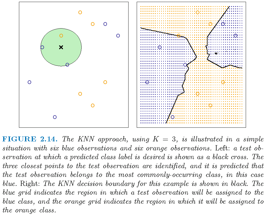
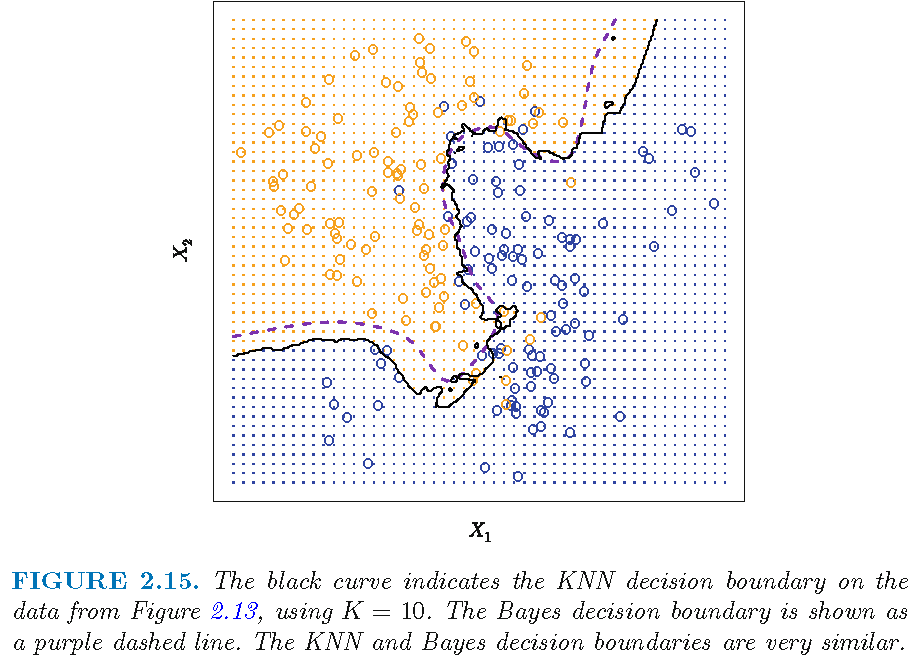
10-NN: decision boundary

200 observations form two distinct groups with equal size

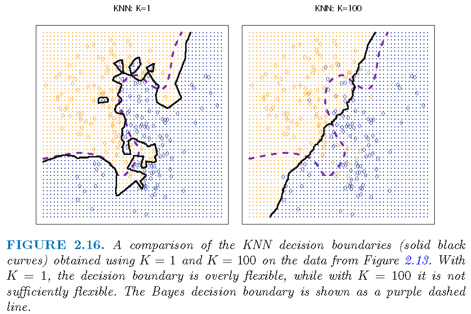
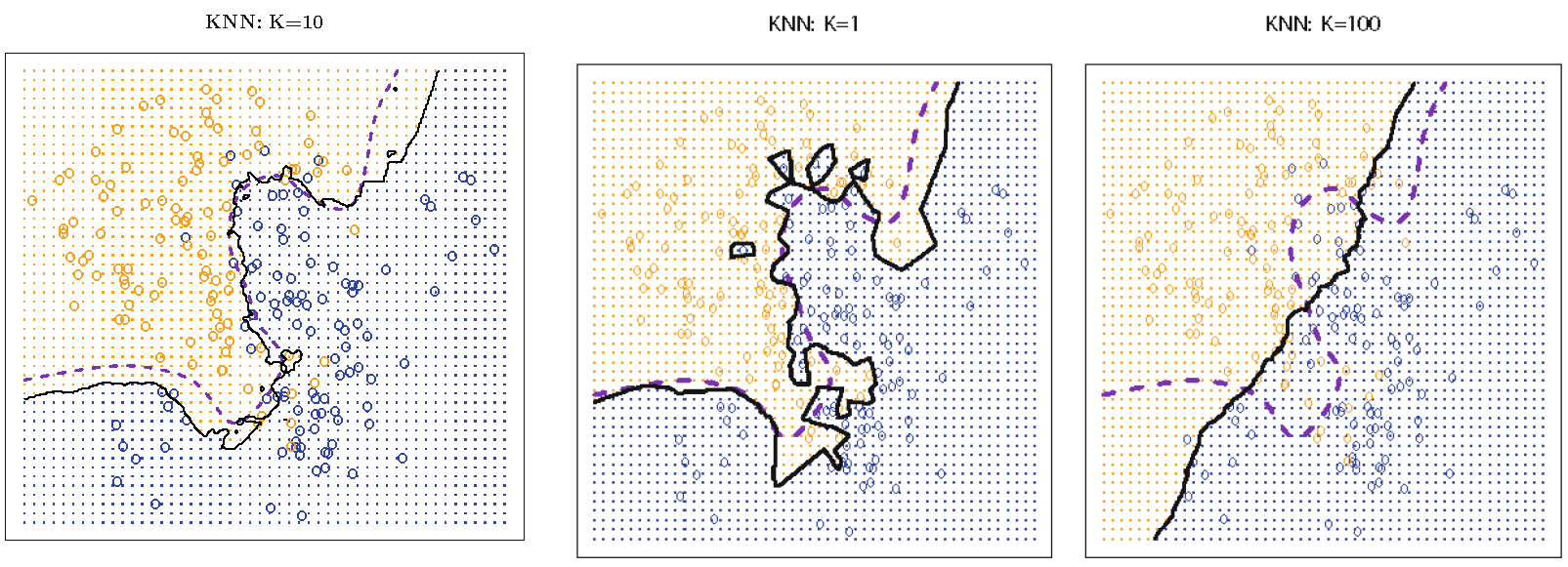
Decision boundaries: k=1 or 100

“flexibility” here refers to “degree of accommodating local properties of features”

kNN: decision boundary

When there are 2 classes, a kNN classifier sets the class label of \(x\) as \[ \hat{Y}(x) = \left\{ \begin{array} {lll} 1 & \text{if} & \bar{Y}(x)=\frac{1}{k}\sum\nolimits_{x_{i}\in N_{k}(x)}y_{i} > 0.5 \\ 0 & \text{if} & \bar{Y}(x)=\frac{1}{k}\sum\nolimits_{x_{i}\in N_{k}(x)}y_{i} \le 0.5 \end{array}\right. \]

• When \(k=1\), there is only 1 training observation \(x_{i'} \in N_{1}(x)\) and \(\bar{Y}(x) = y_{i'}\), the label of \(x_{i'}\), i.e., \(\hat{Y}(x)\) is determined solely by \(y_{i'}\), leading to an “overly flexible” decision boundary that is mostly determined by local properties of features

• So, if we have a complicated data set for classification, then choosing a smaller \(k\) is more sensible

kNN: decision boundary

Recall \(\bar{Y}(x)=\frac{1}{k}\sum\nolimits_{x_{i}\in N_{k}(x)}y_{i}\)

• When \(k\) is much larger than \(1\), then \(\bar{Y}(x)\) is the average of considerably many \(y_{j}\)’s, whose corresponding \(x_{j}\)’s in \(N_{k}(x)\) can span a large subset of the feature space

• So, when two feature observations \(x\) and \(x'\) are not far apart, their neighborhoods \(N_{k}(x)\) and \(N_{k}(x')\) will not contain quite different \(x_{j}\)’s, leading to similar \(\bar{Y}(x)\) and \(\bar{Y}(x')\) and similar \(\hat{Y}(x)\) and \(\hat{Y}(x')\), and a “insufficiently flexible” decision boundary that is relatively smooth

kNN: decision boundary

10 observations form 2 classes (observations 1, 4, 7 and 9 form a class, and the rest form another class):

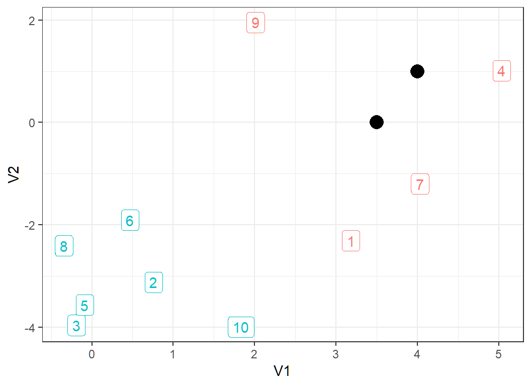
kNN: decision boundary

• Recall that when there are 2 classes, a kNN classifier sets the class label of \(x\) as \[ \hat{Y}(x) = \left\{ \begin{array} {lll} 1 & \text{if} & \bar{Y}(x)=\frac{1}{k}\sum\nolimits_{x_{i}\in N_{k}(x)}y_{i} > 0.5 \\ 0 & \text{if} & \bar{Y}(x)=\frac{1}{k}\sum\nolimits_{x_{i}\in N_{k}(x)}y_{i} \le 0.5 \end{array}\right. \]

• So, it is important (but not easy) to choose a neighborhood size \(k\), not too small and not too large, to obtain good classification performance for a kNN classifier

The 0-1 loss and its expectation

• For an observation \(x\) on the random vector \(X\), let \(Y(x) \in \{0,1\}\) be the true class label of \(x\), and \(\hat{Y}(x) \in \{0,1\}\) the estimated class label for \(x\)

• For \(k,l \in \{0,1\}\), the 0-1 loss \(L\) is defined as: \[L(k,l)=0 \text{ if } k=l \text{ and } L(k,l) =1 \text{ if } k \ne l \] Namely, the loss \(L\) is \(0\) if and only if an observation is correctly classified; otherwise \(L\) is \(1\)

• The expected 0-1 loss is \(\rho=E(L[Y(X),\hat{Y}(X)]),\) where \(E\) denotes expectation. \(\rho\) is unknown in practice and needs to be estimated

Training error and test error

Consider a classifier \(\hat{Y}: x \mapsto \hat{Y}(x) \in \{0,1\}\):

• for the training set \(\mathcal{T}=\{(x_{1},y_{1}),\ldots,(x_{n},y_{n})\}\), write \(\hat{y}_i=\hat{Y}(x_i)\). Then the training error is defined as \[ \varepsilon_n = \frac{1}{n} \sum_{i=1}^n L\left(y_i, \hat{y}_i\right) \] via the 0-1 loss \(L\)
• under certain conditions, we have \(\lim_{n \to \infty} \varepsilon_n = \rho\) with probability \(1\), i.e., with sufficiently many (independent) training observations, the training error approximates well the expected 0-1 loss

Test error

Consider the classifier \(\hat{Y}: x \mapsto \hat{Y}(x) \in \{0,1\}\):

• for a test set \(\mathcal{S}=\{(x_{0i},y_{0i}): i=1,\ldots,m\}\), disjoint with \(\mathcal{T}\) and with unknown class labels \(y_{0i}\in \{0,1\}\), write \(\hat{Y}(x_{0i})=\hat{y}_{0i}\). Then the test error is defined as \[ e_m = \frac{1}{m} \sum_{i=1}^m L\left(y_{0i}, \hat{y}_{0i}\right) \]
• we have \(\lim_{m \to \infty} e_m = \rho\) with probability \(1\) under certain conditions, i.e., with sufficiently many (independent) test observations, the test error approximates well the expected 0-1 loss

Remarks on errors and losses

• The expected 0-1 loss needs to be estimated
• The training error can always be obtained, but the test error may not since we may not have test observations
• Under certain conditions, the expected 0-1 loss can be well approximated by either the training error or the test error; the train error is \(0\) for \(1\)-NN classifier
• The test error is a preferred measure on the performance of a classifier, and a better classifier has a smaller test error
• The Bayes classifier minimizes the expected 0-1 loss

Test error as k changes

Test errors: 0.1304 (Bayes error), 0.1363 (k=10), 0.1695 (k=1), 0.1925 (k=100):

Relative error rates

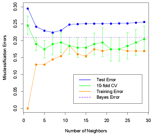
There seems to be a best value for \(k\):

Relative error rates

• It is not necessarily true that a smaller \(k\) leads to a larger test error rate for a kNN classifier

• The training error rate is zero for 1-NN classifier

• There are values of \(k\) for which the corresponding kNN classifiers have the smallest test error rate among a family of kNN classifiers

• The test error rate of a kNN classifier can be close or equal to the Bayes error rate

Relative error rates

\(k=7\) appears to be optimal for minimizing the test error but not for minimizing the cross-validated test error:

A relationship: simple version

For a \(2\)-class problem and class label \(j \in \{0,1\}\),

• logistic regression and the Bayes classifier both compute \[\hat{f}_j(x)=\Pr(Y=j|X=x)\] and assign \(x\) to class \(g\) if \[ \Pr(Y=g|X=x)>0.5 \]

• kNN classifier computes \[\hat{g}_j(x)=k^{-1}\sum\nolimits_{x_{i}\in N_{k}(x)}1\{y_{i}=j\}\]

• when \(k\) is large and \(k/n\) is small,
  \[\hat{g}_j(x) \approx \Pr(Y=j|X=x)\] and the 3 classifiers are similar

A relationship: general version

For a \(K\)-class classification task and \(j \in \mathcal{G}=\{1,\ldots,K\}\),

• logistic regression and the Bayes classifier both compute \[\hat{f}_j(x)=\Pr(Y=j|X=x)\] and assign \(x\) to class \(g\), where \[ g=\operatorname{argmax}\nolimits_{r\in\mathcal{G}}\Pr(Y=r|X=x) \]
• kNN classifier computes \[\hat{g}_j(x)=k^{-1}\sum\nolimits_{x_{i}\in N_{k}(x)}1\{y_{i}=j\}\]
• when \(k\) is large and \(k/n\) is small, \(\hat{g}_j(x) \approx \Pr(Y=j|X=x)\), and all 3 classifiers are similar

Note: \(1\{y_{i}=j\}=1\) if \(y_i=j\) and \(0\) otherwise

Choose k by cross-validation

• The choice of \(k\) can greatly affect the decision boundary and hence classification error of a kNN classifier

• For each data generating process, there seems to be an optimal \(k\) for which the test error of this kNN classifier is minimal among a family of kNN classifiers

• In practice, the choice of \(k\) can be determined by the cross-validation method. However, this method may not provide a good choice of \(k\) when there are insufficient number of observations to use

Neighborhoods in high dimension

Consider observations \(\left\{ x_{i}\right\} _{i=1}^{n}\) for the same \(p\) features, and assume the \(x_i\)’s follow the same probability distribution \(P_{X}\)

• then \(p\) is the dimensionality of the feature space

• Since \(P_{X}\) assigns total mass \(1\) to the feature space, less mass is distributed in each of the \(p\) directions as \(p\) increases. Hence, as \(p\) increases, it is harder to find \(k\) neighboring points around a point \(x\) in the feature space

• Namely, as \(p\) increases, it is harder to construct a \(k\)-point neighborhood \(N_{k}\left( x\right)\). This is related to the curse of dimensionality

License and session Information

License

> sessionInfo()
R version 3.5.0 (2018-04-23)
Platform: x86_64-w64-mingw32/x64 (64-bit)
Running under: Windows 10 x64 (build 19041)

Matrix products: default

locale:
[1] LC_COLLATE=English_United States.1252 
[2] LC_CTYPE=English_United States.1252   
[3] LC_MONETARY=English_United States.1252
[4] LC_NUMERIC=C                          
[5] LC_TIME=English_United States.1252    

attached base packages:
[1] stats     graphics  grDevices utils     datasets  methods  
[7] base     

other attached packages:
[1] knitr_1.21

loaded via a namespace (and not attached):
 [1] compiler_3.5.0  magrittr_1.5    tools_3.5.0    
 [4] htmltools_0.3.6 revealjs_0.9    yaml_2.2.0     
 [7] Rcpp_1.0.0      stringi_1.2.4   rmarkdown_1.11 
[10] stringr_1.3.1   xfun_0.4        digest_0.6.18  
[13] evaluate_0.12