Stat 437 Lecture Notes 4b

Xiongzhi Chen

Washington State University

Bayes classifier: practice

The two-group model

Prior probabilities for class labels: \[\Pr(Y_i =1)=\Pr(Y_i =2)=0.5\]
Conditional density for $x_i$ in Class 1: \[ f_1(x | Y_i=1) \sim \text{Gaussian}(\mu_1=(3,0),\mathbf{I}) \]
Conditional density for $x_i$ in Class 2: \[ f_2(x | Y_i=2) \sim \text{Gaussian}(\mu_2=(0,-4),\mathbf{I}) \]
$n=10$ observations $x_i$’s, which are independent given the $n=10$ class labels $Y_i$

The two-group model

> set.seed(2)
> gp=rbinom(n=10, size=1, prob=0.5)
> gp1=which(gp==0); gp2=which(gp==1) 
> x=matrix(rnorm(10*2), ncol=2)
> x[gp1,1]=x[gp1,1]+3; x[gp2,2]=x[gp2,2]-4

gp=rbinom(...): generate 10 class labels randomly, $0$ for Class 1 and $1$ for Class 2
gp1: indices of observations in Class 1
gp2: indices of observations in Class 2
x[gp1,]: observations from Class 1, with distribution $\text{Gaussian}(\mu_1=(3,0),\mathbf{I})$
x[gp2,]: observations from Class 2, with distribution $\text{Gaussian}(\mu_2=(0,-4),\mathbf{I})$

Generated observations

> colnames(x)=c("V1","V2")
> y = as.data.frame(x); y$obId = 1:10; y$Class=as.factor(gp+1)
> y
           V1        V2 obId Class
1   3.1324203 -2.311069    1     1
2   0.7079547 -3.121395    2     2
3  -0.2396980 -3.964193    3     2
4   4.9844739  1.012829    4     1
5  -0.1387870 -3.567735    5     2
6   0.4176508 -1.909181    6     2
7   3.9817528 -1.199926    7     1
8  -0.3926954 -2.410362    8     2
9   1.9603310  1.954652    9     1
10  1.7822290 -3.995062   10     2

obId: observation id
observation $x_i$ is in row $i$, with coordinates V1 and V2
Class: class label for each $x_i$

Visualize data

> library(ggplot2)
> ggplot(y,aes(V1,V2))+theme_bw()+guides(color = FALSE)+
+   geom_label(aes(label=obId,color=Class))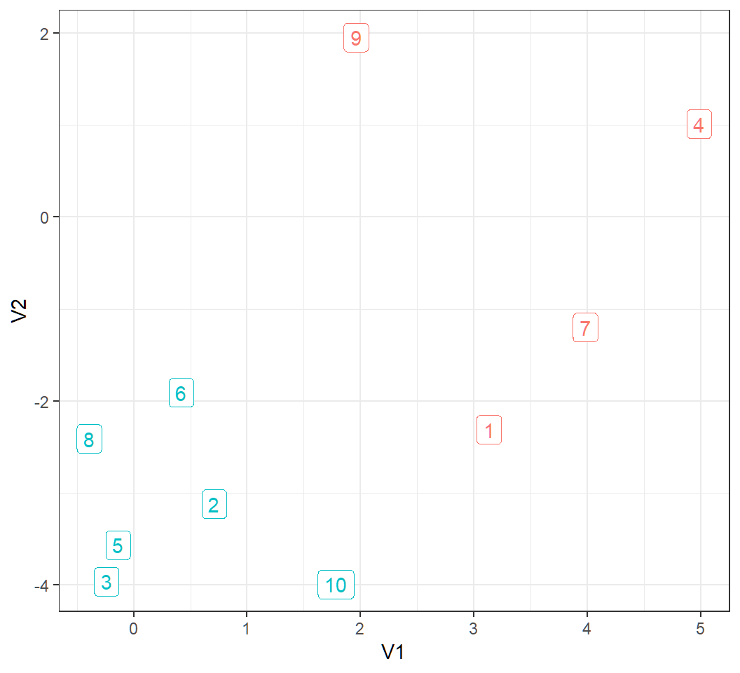

Marginal and posterior distr.

marginal density of $x_i$ is \[ \begin{aligned} f(x) & = f_1(x | Y_i=1) \Pr(Y_i =1) + f_2(x | Y_i=2) \Pr(Y_i =2)\\ & = 0.5f_1(x | Y_i=1) + 0.5 f_2(x | Y_i=2) \end{aligned} \]
posterior probability of $x_i$ belonging to Class $j$ is \[ \begin{aligned} \Pr(Y_i=j|x_i) & = \frac{f_j(x_i | Y_i=j) \Pr(Y_i =j)}{f(x_i)} \\ & = \frac{0.5 f_j(x_i | Y_i=j)}{f(x_i)} \end{aligned} \]
need $f_j(x_i | Y_i=j)$ to get marginal and posterior

Obtain posterior probability

> library(mvtnorm) # compute multivariate Gaussian probabilities
> postPClass = matrix(0,ncol=2,nrow=10) # store prosterior probabilities
> for (i in 1:10) {
+ cndp1 = dmvnorm(x[i,], mean =c(3,0), sigma = diag(2))
+ cndp2 = dmvnorm(x[i,], mean =c(0,-4), sigma = diag(2))
+ fmarginal = 0.5*cndp1 +0.5*cndp2
+ jp1=0.5*cndp1; jp2=0.5*cndp2
+ postp1=jp1/fmarginal; postp2=jp2/fmarginal  
+ postPClass[i,]=c(postp1,postp2)
+ }
> colnames(postPClass)=c("PPCL1","PPCL2")
> postPClass

dmvnorm(x[i,], mean =c(3,0), sigma = diag(2)): $f_1(x_i | Y_i=1) \sim \text{Gaussian}(\mu_1=(3,0),\mathbf{I})$
fmarginal: $f(x_i)$, and jp1: $f_1(x_i | Y_i=1) \Pr(Y_i =1)$
postp1 and postp2: $\Pr(Y_i=1|x_i)$ and $\Pr(Y_i=2|x_i)$

Posterior probabilities

             PPCL1        PPCL2
 [1,] 9.747409e-01 2.525912e-02
 [2,] 1.046019e-03 9.989540e-01
 [3,] 2.095184e-06 9.999979e-01
 [4,] 1.000000e+00 1.683903e-10
 [5,] 1.384877e-05 9.999862e-01
 [6,] 5.296168e-02 9.470383e-01
 [7,] 9.999762e-01 2.380586e-05
 [8,] 6.620328e-04 9.993380e-01
 [9,] 1.000000e+00 3.390852e-08
[10,] 7.972362e-04 9.992028e-01

column 1 PPCL1: posterior probability of an observation belonging to Class 1
column 2 PPCL2: posterior probability of an observation belonging to Class 2

Bayes classifier

Bayes classifier assigns $x_i$ to Class $j$ if $\Pr(Y_i=j|x_i)$ is the larger among the two $\Pr(Y_i=k|x_i)$ for $k=1$ or $2$:

> postPClass=data.frame(postPClass) 
> postPClass$TrueClass = rep(1,10)
> postPClass$TrueClass[gp2]=2 #true class labels
> postPClass$EstClass=rep(1,10)
> # compare posterior probabilities
> comp = (postPClass$PPCL1 >= postPClass$PPCL2) 
> postPClass$EstClass[comp==TRUE]=1 # assign Class 1
> postPClass$EstClass[comp==FALSE]=2 # assign Class 2
> postPClass

postPClass$PPCL1 >= postPClass$PPCL2: check if $\Pr(Y_i=1|x_i)>\Pr(Y_i=2|x_i)$ for each $i$; return a logical vector

Bayes classifier

          PPCL1        PPCL2 TrueClass EstClass
1  9.747409e-01 2.525912e-02         1        1
2  1.046019e-03 9.989540e-01         2        2
3  2.095184e-06 9.999979e-01         2        2
4  1.000000e+00 1.683903e-10         1        1
5  1.384877e-05 9.999862e-01         2        2
6  5.296168e-02 9.470383e-01         2        2
7  9.999762e-01 2.380586e-05         1        1
8  6.620328e-04 9.993380e-01         2        2
9  1.000000e+00 3.390852e-08         1        1
10 7.972362e-04 9.992028e-01         2        2

TrueClass: true class labels
EstClass: labels obtained by the Bayes classifier

Classification error

$\hat{y}_i$: estimated class label for true class label $y_i$ for $x_i$
$L$: 0-1 loss, i.e., $L(y_i,\hat{y}_i)=0$ if $y_i=\hat{y}_i$, and $1$ otherwise

Classification error, defined as \[ e_n = \frac{1}{n} \sum_{i=1}^n L(y_i,\hat{y}_i), \] is zero for this example:

> table(EstClass,TrueClass)
        TrueClass
EstClass 1 2
       1 4 0
       2 0 6

k-nearest neighbor (kNN) classifiers: software implementation

R software needed and workflow

R commands and libraries needed:

R library class and command knn{class} for kNN classification

General workflow for kNN classifiers:

standardize each feature (if measurements on different features are on quite different scales since the Euclidean distance is used as a measure on how close two observations are in the construction of neighborhoods)
choose an optimal neighborhood size $k$ (e.g., by cross-validation)
apply optimal kNN classifier

Command `knn{class}`

knn{class} implements kNN classification for test set from training set:

for each row of the test set, the k nearest vectors (in Euclidean distance) from the training set are found and selected
the classification is decided by majority vote, based on the class labels of the k nearest vectors
if there are ties (in Euclidean distance) for the kth nearest vector among the selected vectors, then all such “tied” vectors are included in the vote

Command `knn{class}`

Its basic syntax is

knn(train, test, cl, k = 1, prob = FALSE)

train: matrix or data frame of training set cases
test: matrix or data frame of test set cases. A vector will be interpreted as a row vector for a single case
cl: factor of true classifications of training set
k: number of neighbors to use
prob: if set as true, the proportion of the votes for the winning class is returned as attribute prob

k-nearest neighbor (kNN) classifiers: Example 1

Generate data

Randomly generate 30 independent observations from a tri-variate Gaussian distribution with mean 0 and identity covariance matrix

> set.seed(1); x=matrix(rnorm(30*3), ncol=3)
> colnames(x) = c("X1","X2","X3"); x = as.data.frame(x)
> x$class= rep(1,nrow(x))

x has 30 rows and 3 columns, i.e., there are 30 observations for 3 features
the 30 observations form 1 class (judged from the distribution they follow)

Visualize data

> library(ggplot2)
> ggplot(data=x,aes(X1,X2,color=X3))+geom_point()+theme_bw()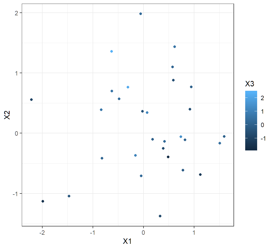

Split data

set the first 20 observations in x as training set
set the rest 10 observations in x as test set

> trainingSet =x[1:20,1:3]; trainingLabels =x[1:20,4]
> testSet =x[21:30,1:3]; testLabels =x[21:30,4]

Note: in terms of software implementation via knn, training set and test set contain observations for features but not class labels

kNN: k=1 or 3

Fact: $k$NN classification error is $0$ for all $k$ when there is only one class (since the average label is always the exact, true class label)

> library(class)
> knn1 = knn(trainingSet,testSet, cl=trainingLabels, k = 1)
> table(knn1,testLabels)
    testLabels
knn1  1
   1 10
> knn3 = knn(trainingSet,testSet, cl=trainingLabels, k = 3)
> table(knn3,testLabels)
    testLabels
knn3  1
   1 10

0 classification error

kNN: k=10 or 30

Fact: $k$NN classification error is $0$ for all $k$ when there is only one class (since the average label is always the exact, true class label)

> library(class)
> knn10 = knn(trainingSet,testSet, cl=trainingLabels, k = 10)
> table(knn10,testLabels)
     testLabels
knn10  1
    1 10
> knn30 = knn(trainingSet,testSet, cl=trainingLabels, k = 30)
> table(knn30,testLabels)
     testLabels
knn30  1
    1 10

0 classification error

kNN: k bigger than sample size

kNN classifier with $k > n$, i.e., neighborhood size bigger than sample size; $n=30$, $k=31$, $k=40$:

> library(class)
> knn(trainingSet,testSet, cl=trainingLabels, k = 31)
Warning in knn(trainingSet, testSet, cl = trainingLabels, k =
31): k = 31 exceeds number 20 of patterns
 [1] 1 1 1 1 1 1 1 1 1 1
Levels: 1
> knn(trainingSet,testSet, cl=trainingLabels, k = 40)
Warning in knn(trainingSet, testSet, cl = trainingLabels, k =
40): k = 40 exceeds number 20 of patterns
 [1] 1 1 1 1 1 1 1 1 1 1
Levels: 1

0 classification error but with warnings
insensible to pick $k >n_1$, where $n_1$ is the sample size for training set

k-nearest neighbor (kNN) classifiers: Example 2

Human cancer microarray data

Human cancer microarray data:

6830 genes (i.e., 6830 features)
64 samples (i.e., 64 cancer cell lines)
14 different cancer types; information on cancer types at wiki-NCI60

The data matrix has dimension $6830 \times 64$, each of whose columns is an observation for all features

We will pick 3 caner types “BREAST”, “LEUKEMIA”, “COLON”, and randomly select the same set of $50$ genes for each cancer type, to balance computations and illustrate kNN classifiers

Obtain subset of data

> library(ElemStatLearn) # library containing data
> data(nci); n = dim(nci)[2]; p = dim(nci)[1] #get dimensions
> set.seed(123)
> rSel = sample(1:p, size=50, replace = FALSE)
> chk = colnames(nci) %in% c("BREAST", "LEUKEMIA", "COLON")
> cSel = which(chk ==TRUE)
> ncia = nci[rSel,cSel]
> colnames(ncia) = colnames(nci)[cSel]

colnames(nci): each column name is the cancer type for an observation
chk: check if a cancer type is “BREAST”, “LEUKEMIA” or “COLON”
take features (i.e., genes) from rows of nci, and take samples (i.e., observations for features) from columns of nci

Glimpse on subset of data

First few entries of the transposed subset data:

> ncib=data.frame(t(ncia)); ncib$Class=colnames(ncia)
> dim(ncib)
[1] 20 51
> head(ncib[1:3,1:5])
             X1     X2    X3     X4     X5
BREAST   -0.075 1.1725 0.510  0.385  0.765
BREAST.1 -0.570 0.0975 0.565 -0.830  2.130
BREAST.2  0.000 1.0375 1.175 -0.160 -0.150

For ncib:

20 rows; 1st 50 entries of each row form an observation for all 50 features
last entry of each row is the cancer type of an observation

Visualize subset of data

> library(ggplot2)
> ggplot(ncib,aes(X1,X2,color=Class))+geom_point()+theme_bw()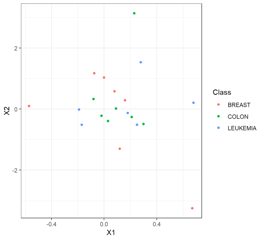

Standardize and split data

60% of standardized data as training set, and the rest 40% as test set:

> ncibsd=scale(ncib[,1:50]); set.seed(1)
> rTrain= base::sample(1:nrow(ncibsd),0.6*nrow(ncibsd))
> rTest =(1:nrow(ncibsd))[-rTrain]
> trainSet =ncibsd[rTrain,]; testSet =ncibsd[rTest,]
> trainLabels=ncib$Class[rTrain]; testLabels=ncib$Class[rTest]

scale(ncib[,1:50]): standardize each feature (i.e., each column) of data
last column of ncib contains class labels

kNN: k=2

> library(class)
> knn2eg2= knn(trainSet,testSet, cl=trainLabels, k = 2)
> length(testLabels)
[1] 8
> testLabels
[1] "LEUKEMIA" "LEUKEMIA" "COLON"    "COLON"    "COLON"   
[6] "BREAST"   "BREAST"   "BREAST"  
> table(knn2eg2,testLabels)
          testLabels
knn2eg2    BREAST COLON LEUKEMIA
  BREAST        1     0        0
  COLON         2     3        0
  LEUKEMIA      0     0        2
> # classification error
> sum(1- as.numeric(knn2eg2==testLabels))/length(testLabels)
[1] 0.25

$8$ test observations; $2$ of them are misclassified (i.e., $2$ observations for “BREAST” cancer are misclassified)
classification error is $2/8=0.25$

kNN: k=4

> library(class)
> knn4eg2= knn(trainSet,testSet, cl=trainLabels, k = 4)
> length(testLabels)
[1] 8
> testLabels
[1] "LEUKEMIA" "LEUKEMIA" "COLON"    "COLON"    "COLON"   
[6] "BREAST"   "BREAST"   "BREAST"  
> table(knn4eg2,testLabels)
          testLabels
knn4eg2    BREAST COLON LEUKEMIA
  BREAST        1     0        0
  COLON         1     2        0
  LEUKEMIA      1     1        2
> # classification error
> sum(1- as.numeric(knn4eg2==testLabels))/length(testLabels)
[1] 0.375

$8$ test observations; $3$ of them are misclassified (i.e., $2$ observations for “BREAST” cancer and $1$ observation for “COLON” cancer are misclassified)
classification error is $3/8=0.375$

Remarks

For the example, the data set we investigated has only $20$ observations. So, it is not very sensible to try cross-validation to choose an optimal neighborhood size $k$

k-nearest neighbor (kNN) classifiers: Example 3

Iris flower data

For each of 3 species “setosa”, “versicolor”, “virginica” of irises, 50 observations on 4 features Sepal.Length, Sepal.Width, Petal.Length and Petal.Width are stored in object iris (in R library ggplot2 or class)

> library(class); dim(iris)
[1] 150   5
> iris[1,]
  Sepal.Length Sepal.Width Petal.Length Petal.Width Species
1          5.1         3.5          1.4         0.2  setosa
> unique(iris$Species)
[1] setosa     versicolor virginica 
Levels: setosa versicolor virginica

The target is to classify an iris plant into one of the three species using these measurements

Data splitting and cross-validation

Proposal for data splitting and cross-validation (cv):

80% of data as training set that contains 40 random samples for each species, and the rest 20% as test set
apply “$m$-fold cross-validation” on the training set to choose optimal $k$ for kNN classifiers
apply optimal kNN classifier to test set

Note: different proportions can be used for data splitting, and they should ensure that a learning method be well trained; usually 5-fold or 10-fold cross-validation is used

Estimating test error

We cannot directly estimate test error using test set since we do not know the class labels for observations in this set
So, we split the training set into 2 disjoint subsets: one as “training set” and the other as “test set”, for which we know the class labels for their observations, and test error is estimated using such “test set”; namely, part of the training set is used as a test set
$m$-fold cross-validation implements the above strategy by randomly splitting the training set into $m$ folds of approximately equal size, uses 1 fold as “test set” and the rest as “training set”, and does this for each of the $m$ folds; see Chapter 5 of Text for details on cross-validation

Splitting data: Step 0

> library(class); set.seed(314) # seed needed!!
> trainId=c(sample(1:50,40),sample(51:100,40),
+           sample(101:150,40))
> testId = (1:150)[-trainId]
> trainingSet=iris[trainId,1:4]; testSet=iris[testId,1:4]
> trainingLabs=iris$Species[trainId]
> testLabs=iris$Species[testId]

trainId=c(...): observation id’s for training set; in data matrix iris, 1st 50 rows (i.e., observations) are for “setosa”, 2nd 50 for “versicolor”, and 3rd 50 for “virginica”
trainingSet contains 40 random samples for each species; testSet is the test set
trainingLabs (or testLabs): class labels for observations in training set (or tet set)

Cross-validation: Step 1

$10$-fold random split of training set:

> m=10; set.seed(123) # seed needed!!
> nrow(trainingSet)
[1] 120
> folds=sample(1:m,nrow(trainingSet),replace=TRUE)
> folds[1:10]
 [1]  3  8  5  9 10  1  6  9  6  5

folds=sample(...,replace=TRUE): sample with replacement (i.e., replace=TRUE) entries of the vector $(1,2,\ldots,m)$ 120=nrow(trainingSet) times, and store sampled entries into folds
folds has 120=nrow(trainingSet) entries, and the entries are numbers between $1$ and $m=10$ and can be repeated

Cross-validation: Step 1 (cont’d)

> which(folds==1) # obs. id's in fold 1
[1]   6  18  35  51  62  74  98 113
> table(folds)
folds
 1  2  3  4  5  6  7  8  9 10 
 8 14 11 11 18 10 12 12 12 12

for each s between 1 and $m$, which(folds==s) returns the id’s of observations in fold s
table(folds) shows, in the 2nd row of its output, the number of observations in each fold (with fold number stored in folds), which equivalently checks if folds have approximately equal size

Cross-validation: Step 2

$10$-fold cv for 2-NN classifier on training Set:

> k=2 # k for kNN; m=10 
> testError1 = double(m) # store test error for each fold s 
> for (s in 1:m) {  # loop through s=1,...,m
+   trainingTmp =trainingSet[folds !=s,]
+   testTmp =trainingSet[folds==s,]
+   trainingLabsTmp =trainingLabs[folds !=s] 
+   testLabsTmp =trainingLabs[folds==s]
+   knn2= knn(trainingTmp,testTmp,trainingLabsTmp,k)
+   nOfMissObs= sum(1-as.numeric(knn2==testLabsTmp))
+   terror=nOfMissObs/length(testLabsTmp) # test error
+   testError1[s]=terror  
+   } # end of loop

for each s, fold s, i.e., testTmp, is “test set” with class labels testLabsTmp, and other folds, i.e., trainingTmp, is “training set” with class labels trainingLabsTmp

Cross-validation: Step 2 (cont’d)

>  mean(testError1)
[1] 0.05040404
>  sd(testError1)
[1] 0.04484363

testError1: a vector of $m$ entries, whose $s$th entry is the estimated test error obtained by setting fold s as test set, as s changes from 1 to $m$
the sample mean of all $m$ entries of testError1 is regarded as the estimated test error for the given kNN classifier (k=2 in the example codes)

Cross-validation: summary

Summary for $m$-fold cross-validation for a kNN classifier:

Randomly split $n$ observations into $m$ folds of approximately equal size
Pick fold $s$ as “test set”, set the remaining folds as “training set”, apply the kNN classifier, and obtain test error $e_{s}$
Do Item 2. for each $s$ in $\{1,\ldots,m\}$, and obtain $m$ $e_{s}$’s
Compute sample mean $\hat{\mu}(k,m)$ and sample standard deviation $\hat{\sigma}(k,m)$ for the $m$ $e_{s}$’s
Use $\hat{\mu}(k,m)$ as an estimate of the test error of the classifier

Note: we call $e_{s}$ “test error” even though it is an estimate of test error

Cross-validation: Step 3

Choose optimal $k$ via $m$-fold cross-validation for kNN classifiers using training set:

Pick a sequence $C$ of $b$ distinct values for $k$
Do Step 1 and Step 2 for each $k$ in $C$, obtain $b$ estimated test errors, $\hat{\mu}(k,m), k \in C$, for the $b$ kNN classifiers
Set as the optimal $\hat{k}$ for which $\hat{\mu}(\hat{k},m)$ is the smallest among $\hat{\mu}(k,m), k \in C$, i.e., \[\hat{k} = \operatorname*{argmin}\{k \in C: \hat{\mu}(k,m)\}\]

Note: if we have enough computational power, we can pick $C=\{1,2,\ldots,k_{\max}\}$ for a large number $k_{\max}$

Cross-validation: Step 3 (cont’d)

If there are multiple optimal $\hat{k}$’s, then set the optimal as the one whose corresponding estimated test error has the smallest sample standard deviation for these optimal kNN classifiers
For example, if $\hat{\mu}(\hat{k}_1,m)$ and $\hat{\mu}(\hat{k}_2,m)$ are both the smallest among $\hat{\mu}(k,m), k \in C$ but $\hat{\sigma}(\hat{k}_1,m) < \hat{\sigma}(\hat{k}_2,m)$, then pick $\hat{k}_1$ as the optimal
If further the estimated test errors of the kNN classifiers with these optimal $\hat{k}$’s have the same sample standard deviation, then pick the optimal as the smallest among these $\hat{k}$ (which can reduce the computational cost of building neighborhoods for the optimal kNN classifier)

Cross-validation: Step 3

$10$-fold cv for kNN classifiers for $k=1,\ldots,20$:

> kmax=20 # m=10 fold cv
> testErrors = matrix(0,nrow=2,ncol=kmax)
> for (k in 1:kmax) { # loop through k
+ testError1 = double(m) # store test errors for each k
+ for (s in 1:m) {  # loop through s
+   trainingTmp =trainingSet[folds !=s,]
+   testTmp =trainingSet[folds==s,]
+   trainingLabsTmp =trainingLabs[folds !=s] 
+   testLabsTmp =trainingLabs[folds==s]
+   knntmp= knn(trainingTmp,testTmp,trainingLabsTmp,k)
+   nOfMissObs= sum(1-as.numeric(knntmp==testLabsTmp))
+   terror=nOfMissObs/length(testLabsTmp) # test error
+   testError1[s]=terror    } # loop in s ends 
+ testErrors[,k]=c(mean(testError1),sd(testError1)) 
+ } # loop in k ends

testErrors: each column contains the sample mean and sample standard deviation for the estimated test errors for a kNN classifier as $k$ varies from $1$ to kmax

Cross-validation: Step 3 (cont’d)

Optimal $\hat{k}$ chosen by $10$-fold cv for $k=1,\ldots,20$:

> colnames(testErrors)= paste("k=",1:kmax,sep="")
> rownames(testErrors)=c("mean(TestError)","sd(TestError)")
> testErrors=as.data.frame(testErrors)
> as.numeric(testErrors[1,])
 [1] 0.04088023 0.04643579 0.04802309 0.03337662 0.03337662
 [6] 0.03893218 0.03456710 0.04012266 0.03178932 0.03532468
[11] 0.04088023 0.04088023 0.04921356 0.04365801 0.05476912
[16] 0.04088023 0.04088023 0.04921356 0.05476912 0.04088023
> hatk=which(testErrors[1,]==min(testErrors[1,]))
> hatk
[1] 9

hatk=which(...): find optimal $\hat{k}$ for which the sample mean of the estimated test error is the smallest as $k$ varies from $1$ to kmax; the optimal $\hat{k}=9$

Cross-validation: extra

If we want to do $m$-fold cross-validation for kNN classifiers with $k$ values in a sequence $C$ using a different $m$-fold split of the training set, we only need to

Do Step 0 with a different set.seed value to get different folds via the command sample, and then
Do Step 1, 2 and 3

Apply optimal kNN classifier

Apply optimal classifier to test set:

> library(class)
> knnOpt= knn(trainingSet,testSet,trainingLabs,hatk)
> nOfMissObs1= sum(1-as.numeric(knnOpt==testLabs))
> terrorOpt=nOfMissObs1/length(testLabs) # test error
> terrorOpt  
[1] 0
> table(knnOpt,testLabs)
            testLabs
knnOpt       setosa versicolor virginica
  setosa         10          0         0
  versicolor      0         10         0
  virginica       0          0        10

hatk: the optimal $\hat{k}=9$ obtained by $10$-fold cross-validation on training set trainingSet
original training set trainingSet is used by the optimal $9$-NN classifier to classify observations in testSet

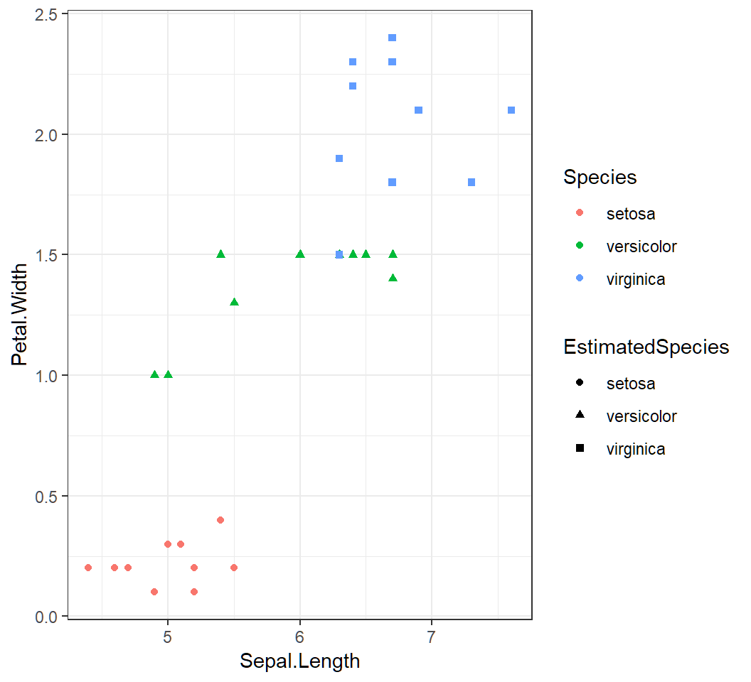
Visualization via 2 features

> testSet$Species=testLabs
> testSet$EstimatedSpecies=knnOpt
> library(ggplot2)
> cp =ggplot(testSet,aes(Sepal.Length,Petal.Width))+
+   geom_point(aes(shape=EstimatedSpecies,color=Species))+
+   theme_bw()

add to testSet the true Species labels and estimated species labels EstimatedSpecies
create plot by ggplot using features Sepal.Length and Petal.Width with shape and color aesthetics

Visualization via 2 features

Perfect classification:

License and session Information

License

> sessionInfo()
R version 3.5.0 (2018-04-23)
Platform: x86_64-w64-mingw32/x64 (64-bit)
Running under: Windows 10 x64 (build 19041)

Matrix products: default

locale:
[1] LC_COLLATE=English_United States.1252 
[2] LC_CTYPE=English_United States.1252   
[3] LC_MONETARY=English_United States.1252
[4] LC_NUMERIC=C                          
[5] LC_TIME=English_United States.1252    

attached base packages:
[1] stats     graphics  grDevices utils     datasets  methods  
[7] base     

other attached packages:
[1] knitr_1.21

loaded via a namespace (and not attached):
 [1] compiler_3.5.0  magrittr_1.5    tools_3.5.0    
 [4] htmltools_0.3.6 revealjs_0.9    yaml_2.2.0     
 [7] Rcpp_1.0.0      stringi_1.2.4   rmarkdown_1.11 
[10] stringr_1.3.1   xfun_0.4        digest_0.6.18  
[13] evaluate_0.12

Stat 437 Lecture Notes 4b

Xiongzhi Chen

Washington State University

Bayes classifier: practice

The two-group model

The two-group model

Generated observations

Visualize data

Marginal and posterior distr.

Obtain posterior probability

Posterior probabilities

Bayes classifier

Bayes classifier

Classification error

k-nearest neighbor (kNN) classifiers: software implementation

R software needed and workflow

Command knn{class}

Command knn{class}

k-nearest neighbor (kNN) classifiers: Example 1

Generate data

Visualize data

Split data

kNN: k=1 or 3

kNN: k=10 or 30

kNN: k bigger than sample size

k-nearest neighbor (kNN) classifiers: Example 2

Human cancer microarray data

Obtain subset of data

Glimpse on subset of data

Visualize subset of data

Standardize and split data

kNN: k=2

kNN: k=4

Remarks

k-nearest neighbor (kNN) classifiers: Example 3

Iris flower data

Data splitting and cross-validation

Estimating test error

Splitting data: Step 0

Cross-validation: Step 1

Cross-validation: Step 1 (cont’d)

Cross-validation: Step 2

Cross-validation: Step 2 (cont’d)

Cross-validation: summary

Cross-validation: Step 3

Cross-validation: Step 3 (cont’d)

Cross-validation: Step 3

Cross-validation: Step 3 (cont’d)

Cross-validation: extra

Apply optimal kNN classifier

Visualization via 2 features

Visualization via 2 features

License and session Information

Command `knn{class}`

Command `knn{class}`