Overview

Discriminant analysis is a classification technique that

• employs a Gaussian mixture model to model data
• approximates the Bayes classifier in the setting of Gaussian mixture models

Contents in Text or Supp. Text

The contents on discriminant analysis are adapted or adopted from:

• mainly Chapter 4 of the Text “An Introduction to Statistical Learning with Applications in R (Corrected at 8th printing)”

• partially Chapter 4 of the Supplementary Text “The Elements of Statistical Learning: Data Mining, Inference, and Prediction (2nd Edition)”

• other sources

Structure of learning module

Structure of learning module on discriminant analysis:

• Review on logistic regression for classification

• Review on Bayes classifiers

• Discriminant analysis via Gaussian mixture models

• Software implementation of discriminant analysis

Classification task

Training set \(\mathcal{T}\) of \(n\) observations \((x_{1},y_{1}),\ldots,(x_{n},y_{n})\)

• \(x_{i}\in \mathbb{R}^{p}\) records the \(i\)th observation for the same \(p\) features
• \(y_{i}\in \mathcal{G}=\{1,\ldots,K\}\) is the class label for \(x_{i}\), and \(1, \ldots, K\) are the class labels

The task: for a new observation (i.e., test observation) \((x_0,y_0)\) with known \(x_0\in\mathbb{R}^{p}\) but unknown \(y_0\in \mathcal{G}\), estimate the class label \(y_0\) of \(x_0\), i.e., classify \(x_0\) into one of the \(K\) classes

Modelling log-odds: K=2

• Let random variable \(X_j\) denote feature \(j\) and \(X=(X_1,X_2,\ldots,X_p)\)
• Let \(Y\), written also as \(Y(X)\), be the class label for \(X\)
• Let \(p_1(x)\) be the probability of an observation \(x\) (from \(X\)) being in Class \(1\), i.e., \(p_1(x) = \Pr(Y=1|X=x)\)

When \(K=2\), i.e., there are 2 classes, logistic regression models the log-odds (or logit) as \[ \log\left(\frac{p_1(X)}{1-p_1(X)}\right) = \beta_0 + \beta_1 X_1 + \cdots+\beta_p X_p \] and estimates the parameter vector \(\boldsymbol{\beta}=(\beta_0,\beta_1,\ldots,\beta_p)\) using the training set \(\mathcal{T}\)

Baseline class: K=2

• Since \(p_1(x) = \Pr(Y=1|X=x)\), then when there are 2 classes, the probability of \(x\) being in Class \(2\) is \[p_2(x)=1-p_1(x)=\Pr(Y=2|X=x)\]
• So, logistic regression models the logit \[ \log\left(\frac{p_1(X)}{1-p_1(X)}\right) = \log\left(\frac{p_1(X)}{p_2(x)}\right), \] where \(p_2(x)\) is taken as the baseline

Caution: Logistic regression does NOT employ a Bayesian model, i.e., no prior probabilities are imposed on the class label \(Y(x')\) such that \(\Pr(Y(x')=1)=p\) for some \(p \in (0,1)\) for all \(X=x'\)

Predicting class labels: K=2

• The parameter vector \(\boldsymbol{\beta}\) is often estimated by the method of maximum likelihood, and the resulting estimate is usually called maximum likelihood estimate (MLE)
• With an estimate \(\hat{\boldsymbol{\beta}}=(\hat{\beta}_0,\hat{\beta}_1,\ldots,\hat{\beta}_p)\) of \(\boldsymbol{\beta}\), \(p_1(X) = \Pr(Y=1|X)\) is estimated by \[ \hat{p}_1(X) = \frac{ \exp{(\hat{\beta}_0+\hat{\beta}_1 X_1+\cdots+\hat{\beta}_p X_p)} } {1+\exp{(\hat{\beta}_0+\hat{\beta}_1 X_1+\cdots+\hat{\beta}_p X_p)}} \]
• Let \(\hat{Y}(x_0)\) be the estimated class label for \(x_0\). Then logistic regression sets \(\hat{Y}(x_0)=1\) if \(\hat{p}_1(x_0)>0.5\), and \(\hat{Y}(x_0)=2\) otherwise

Penalized version: K=2

• Given \(n\) observations \(x_{i}\) for \(X\), and class labels \(y_i\) for \(Y\), such that \(y_i \in \{0,1\}\)’s are independent from \(x_{i}\)’s, the likelihood function for the parameter vector \(\boldsymbol{\beta}\) is \[ L\left( \boldsymbol{\beta}\right) =\prod\nolimits_{i=1}^{n}p_{i}^{y_{i}}\left( 1-p_{i}\right) ^{1-y_{i}} \quad \text{with} \quad p_{i}=p_1(x_{i}) \]

• When \(p > n\), the logistic regression model is unstable, and its penalized version, such as LASSO logistic regression or Ridge logistic regression, is often used

• LASSO logistic regression: \[ \hat{\boldsymbol{\beta}} \in\operatorname*{argmin}_{\boldsymbol{\beta}}\left[ -\log L\left( {\boldsymbol{\beta}}\right) +\lambda\sum_{j=1}^{p}\left\vert \beta_{j}\right\vert \right], \lambda \ge 0 \]

Penalized version: K=2

• Ridge logistic regression: \[ \hat{\boldsymbol{\beta}} \in\operatorname*{argmin}_{{\boldsymbol{\beta}}}\left[ - \log L\left( {\boldsymbol{\beta}}\right) +\lambda\sum_{j=1}^{p}\left\vert \beta_{j}\right\vert ^{2}\right], \lambda \ge 0 \]

• Let \(\hat{Y}(x_0)\) be the estimated class label for \(x_0\). Then logistic regression sets \(\hat{Y}(x_0)=1\) if \(\hat{p}_1(x_0)>0.5\), and \(\hat{Y}(x_0)=2\) otherwise

Note: \(\operatorname*{argmin}_{\boldsymbol{\beta}}\) is the set of \(\boldsymbol{\beta}\) values which minimize the corresponding objective function

Modelling log-odds: K>2

• For each \(k=1,\ldots,K-1\), logistic regression models the logit \(r_{k}(X)\) as \[ \begin{aligned} r_{k}(X) &=\log\left[\frac{\Pr(Y=k|X)}{\Pr(Y=K|X)}\right] \\ & =\beta_{k0}+\beta_{k1}X_1+\cdots+\beta_{kp}X_p \end{aligned} \] and uses the training set \(\mathcal{T}\) to estimate each parameter vector \[\boldsymbol{\beta}_k=(\beta_{k0}, \beta_{k1},\ldots,\beta_{kp}), k=1,\ldots,K-1\]
• Here \(\Pr(Y=K|X)\) is used as the baseline

Caution: no prior probability is put on \(Y(X)=k\) for each \(k=1,\ldots,K\)

Predicting class labels: K>2

• The long parameter vector \(\boldsymbol{\beta}=(\boldsymbol{\beta}_1,\ldots,\boldsymbol{\beta}_{K-1})\) (containing the \(K-1\) vectors \(\boldsymbol{\beta}_k,k=1,\ldots,K-1\) and with \((p+1)\times (K-1)\) entries) is often estimated by the method of maximum likelihood

• Let an estimate of \(\boldsymbol{\beta}\) be \(\boldsymbol{\hat{\beta}}=(\boldsymbol{\hat{\beta}}_1,\ldots,\boldsymbol{\hat{\beta}}_{K-1})\) with \(\boldsymbol{\hat{\beta}}_k=(\hat{\beta}_{k0},\hat{\beta}_{k1},\ldots,\hat{\beta}_{kp}),k=1,\ldots,K-1\)

• For each \(k=1,\ldots,K-1\), the estimate \(\boldsymbol{\hat{\beta}}_k\) gives an estimate of \(p_k(X) = \Pr(Y=k|X)\) as \[ \hat{p}_k(X) = \frac{ \exp{(\hat{\beta}_{k0}+\hat{\beta}_{k1} X_1+\cdots+\hat{\beta}_{kp} X_p)} } {1+\sum_{l=1}^{K-1}\exp{(\hat{\beta}_{l0}+\hat{\beta}_{l1} X_1+\cdots+\hat{\beta}_{lp} X_p)}} \]

Predicting class labels: K>2

• Note that \(p_K(X) = \Pr(Y=K|X)\) is estimated as \[ \hat{p}_K(X) = \frac{ 1 } {1+\sum_{l=1}^{K-1}\exp{(\hat{\beta}_{l0}+\hat{\beta}_{l1} X_1+\cdots+\hat{\beta}_{lp} X_p)}} \]

• Let \(\hat{Y}(x_0)\) be the estimated class label for \(x_0\). Then logistic regression sets \(\hat{Y}(x_0)=g\) if \[\hat{p}_{g}(x_0) = \max\{\hat{p}_k(x_0):k=1,\ldots,K\}\]

Note: \(\Pr(Y=k|X)\) for any \(k \in \{1,\ldots,K\}\) can be set as the baseline

Classification task

Training set \(\mathcal{T}\) of \(n\) observations \((x_{1},y_{1}),\ldots,(x_{n},y_{n})\)

• \(x_{i}\in \mathbb{R}^{p}\) records the \(i\)th observation for the same \(p\) features
• \(y_{i}\in \mathcal{G}=\{1,\ldots,K\}\) is the class label for \(x_{i}\), i.e., \(1, \ldots, K\) are the class labels

The task: for a new observation (i.e., test observation) \((x_0,y_0)\) with known \(x_0\in\mathbb{R}^{p}\) but unknown \(y_0\in \mathcal{G}\), estimate the class label \(y_0\) of \(x_0\), i.e., classify \(x_0\) into one of the \(K\) classes

Bayesian modelling

• The observations on the \(p\) features, i.e., \(x_i\)’s, are regarded as a sample from a random vector \(X \in \mathbb{R}^p\)

• The class labels, i.e., \(y_i\)’s, are regarded as a sample from a random variable \(Y\), to capture the hypothesis that for each observation \(x'\) from \(X\), its class label \(Y'\) is random

• The performance of a classifier is measured by how well it classifies new observations on avarage, by accounting for the randomness of \(X\) and \(Y\) when new observations are obtained

Note: in Bayesian modelling, decisions are made using posteriors

Mixture model

Classification based on Bayesian modelling often employs the multi-group mixture model. Suppose there are \(K\) classes, intuitively we model the data generating process as follows:

• Step 1: randomly pick one of the \(K\) classes, such that Class \(l\) has probability \(\pi_l \in (0,1)\) to be picked

• Step 2: generate an observation \(x'\) using distribution or density \(f_k\) if Class \(k\) has bee picked, such that observations in the same class follow the same distribution

• Step 3: repeat Step 1 and Step 2 until a desired number of observations are generated

K-group mixture model

\(K\)-group mixture model with class label set \(\mathcal{G}=\{1,\ldots,K\}\) is given as follows: for each \(k \in \mathcal{G}\),

• prior probability that \(X\) comes from Class \(k\): \[\pi_{k}=\Pr\left(Y=k\right)\]
• conditional density for \(X\) if \(X\) comes from Class \(k\): \[f_{k}\left( x\right) =\Pr\left( X=x|Y=k\right)\]

Note: \(\min_{1\leq i\leq K}\pi_{i}>0\) (otherwise at least one class does not exist) and \(\sum_{i=1}^{K}\pi_{i}=1\) (otherwise we did not sample from at least one class)

Marginal and posterior

For a \(K\)-group mixture model,

• marginal density for \(X\) is \[f\left( x\right) =\pi_{1}f_{1}\left( x\right)+\cdots+\pi_{K}f_{K}\left( x\right),\] and \(X\) is said to have “a mixture density with mixing proportions \(\left\{ \pi_{i}\right\} _{i=1}^{K}\) and components \(\left\{ f_{i}\right\} _{i=1}^{K}\)”

• posterior: \[ \Pr\left( Y=k|X=x\right) =\frac{\pi_{k}\left( x\right) f_{k}\left( x\right) }{f\left( x\right)}, \forall k=1,\ldots,K \] Note: the above expression is the Bayes theorem

The expected 0-1 loss

• Let \(Y(X)\) and \(\hat{Y}(X)\in \{1,\ldots,K\}\) respectively be the true and estimated class label of \(X\)

• For \(k,l \in \{1,\ldots,K\}\), the 0-1 loss \(L\) is defined as \[L(k,l)=0 \text{ if } k=l \text{ and } L(k,l) =1 \text{ if } k \ne l. \] Namely, the 0-1 loss \(L\) is \(0\) if an observation is correctly classified; otherwise \(L\) is \(1\).

• The expected 0-1 loss is \(\rho=E(L[Y(X),\hat{Y}(X)]),\) where \(E\) denotes expectation with respect to the joint distribution of \((X,Y)\)

Bayes classifier

• The Bayes classifier minimizes the expected 0-1 loss

• The Bayes classifier classifies an observation into the class for which the corresponding posterior probability for the observation to belong to this class is the largest among all such posterior probabilities

• Namely, \(X\) is classified into Class \(g\) if \[ g = \operatorname*{argmax}\{k\in \{1,\ldots,K\}: \Pr(\hat{Y}(X)=k|X)\}, \] where \(\hat{Y}(X)\) is the estimated class label for \(X\)

Note: \(\operatorname*{argmax}\) returns the argument at which the maximum being sought is obtained

Bayes classifier in general

• The decision boundary of a Bayes classifier is not necessarily a linear function of the feature variables

• To implement a Bayes classifier, we need the marginal and posterior probabilities of the associated Bayesian model. But in practice, these probabilities need to be estimated

• The error rate of a Bayes classifier often serves as an unattainable gold standard against which to compare other classifiers

Overview

Discriminant analysis

• employs a Gaussian mixture model
• estimates this model and approximates the Bayes classifier in this setting
• has a decision boundary that is determined by the covariance matrix for the feature variables
• is more stable than logistic regression when classes are well-separated or when the number of training observations is small for each class

Classification task

Training set \(\mathcal{T}\) of \(n\) observations \((x_{1},y_{1}),\ldots,(x_{n},y_{n})\)

• \(x_{i}\in \mathbb{R}^{p}\) records the \(i\)th observation for the same \(p\) features
• \(y_{i}\in \mathcal{G}=\{1,\ldots,K\}\) is the class label for \(x_{i}\), i.e., \(1, \ldots, K\) are the class labels

The task: for a new observation (i.e., test observation) \((x_0,y_0)\) with known \(x_0\in\mathbb{R}^{p}\) but unknown \(y_0\in \mathcal{G}\), estimate the class label \(y_0\) of \(x_0\), i.e., classify \(x_0\) into one of the \(K\) classes

Gaussian mixture: p=1

When there is only \(p=1\) feature \(X=X_1\), the \(K\)-group Gaussian mixture model is obtained by setting in the \(K\)-group mixture model

• conditional density \(f_k\) for \(X\) when it comes from Class \(k\) as the Gaussian density with mean vector \(\mu_k\) as the scalar \(\mu_k\) and covariance matrix \(\Sigma_k\) as the scalar \(\sigma_k^2\)

• i.e., by setting \[ \begin{aligned} f_k(x) & \sim \text{Gaussian}(\mu_k,{\Sigma}_k) \\ & = \frac{1}{\sqrt{2\pi} \sigma_k} \exp\left(-\frac{1}{2\sigma_k^2}(x-\mu_k)^2\right) \end{aligned} \]

Gaussian mixture: p>1

When there are \(p>1\) features, the \(K\)-group Gaussian mixture model is obtained by setting

• conditional density \(f_k\) of \(X\) when it comes from Class \(k\) as the Gaussian density with mean vector \(\mu_k\) and \(p \times p\) covariance matrix \(\Sigma_k\)

• i.e., by setting \[ \begin{aligned} f_k(x) & \sim \text{Gaussian}(\mu_k,{\Sigma}_k)\\ & = {\left( 2\pi\right) ^{-p/2}\left\vert\Sigma_{k}\right\vert ^{-1/2}} \exp\left( -\frac{1}{2}\left( x-\mu_{k}\right) ^{T}\Sigma_{k}^{-1}\left( x-\mu_{k}\right) \right), \end{aligned} \] where \(\left\vert\Sigma_{k}\right\vert\) is the determinant of \({\Sigma}_k\) and \(\Sigma_{k}^{-1}\) the inverse of \({\Sigma}_k\), and the superscript \(^T\) means “transpose”

Posterior and classification rule

• Posterior of \(X=x\) belonging to Class \(k\) is \[ q_k(x)=\Pr(Y=k|X=x) = \frac{f_k(x) \Pr(Y =k)}{f(x)} \]
• By simple algebra, we have the log-posterior as \[ \begin{aligned} \log q_k(x) & =-\log\left[ \left( 2\pi\right) ^{p/2}\left\vert \Sigma_{k}\right\vert ^{1/2}\right] +\log\pi_{k}-\log f\left( x\right) \\ & -\frac{1}{2}x^{T}\Sigma_{k}^{-1}x+x^{T}\Sigma_{k}^{-1}\mu_{k}-\frac{1}{2}\mu_{k}^{T}\Sigma_{k}^{-1}\mu_{k} \end{aligned} \]
• Classification rule: \(X=x_0\) is classified into Class \(g\) if \(q_g(x_0)\) (or \(\log q_g(x_0)\)) is the largest among all \(q_k(x_0),k\in\mathcal{G}\) (or \(\log q_g(x_0),k\in\mathcal{G}\))

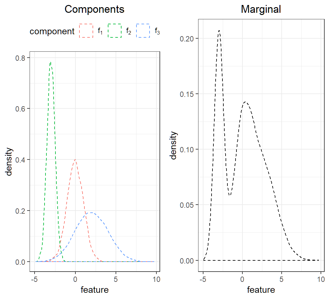
Gaussian mixture: K=3,p=1

Gaussian mixture for \(K=3\) classes and \(p=1\) feature with

• mixing proportions: \(\pi_1=0.2\), \(\pi_2=0.3\), \(\pi_3=0.5\)

• components: \[f_1(x)\sim \text{Gaussian}(0,1),\] \[f_2(x)\sim \text{Gaussian}\left(-3,0.5^2\right)\] and \[f_3(x)\sim \text{Gaussian}\left(2,2^2\right)\]

• marginal: \(f(x)= \sum_{k=1}^3 \pi_k f_k(x)\)

Caution: marginal is not Gaussian

Gaussian mixture: K=3,p=1

Visualization of the Gaussian mixture:

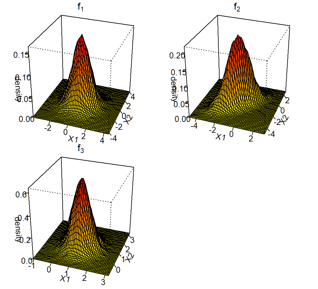
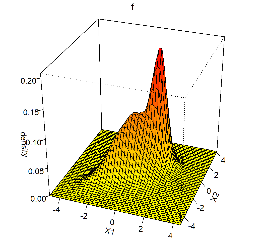
Gaussian mixture: K=3,p=2

Gaussian mixture for \(K=3\) classes and \(p=2\) features with

• mixing proportions: \(\pi_1=0.4\), \(\pi_2=0.3\), \(\pi_3=0.3\)

• components: \[f_1(x)\sim \text{Gaussian}(\mu_1=(0,0)^T,\Sigma_1=\mathbf{I}),\] \[f_2(x)\sim \text{Gaussian}\left(\mu_2=(-1,-1)^T,\Sigma_2=\left(\begin{array}{cc} 1 & 0.7\\ 0.7 & 1 \end{array}\right)\right)\] and \[f_3(x)\sim Gaussian\left(\mu_3=(1,1)^T,\Sigma_3=0.25\mathbf{I}\right)\]

• marginal: \(f(x)= \sum_{k=1}^3 \pi_k f_k(x)\) (not Gaussian)

Note: vectors are column vectors

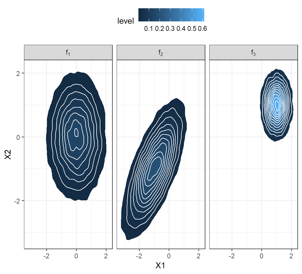
Gaussian density in general

For feature vector \(X \sim \text{Gaussian}(\mu,\Sigma)\),

• \(\mu\) controls the center of sample points from \(X\)

• \(\Sigma\) controls shapes of probability contours: when \(\Sigma=\mathbf{I}\), contours are circles; when \(\Sigma \ne \mathbf{I}\), contours are ellipses

• \(\Sigma\) controls correlations: when \(\Sigma=\mathbf{I}\), feature variables are uncorrelated; when \(\Sigma \ne \mathbf{I}\), feature variables are correlated

• \(\Sigma\) controls the density peak height and concentration of density: smaller \(\Sigma\) (in terms of its eigenvalues) gives larger peak height and more concentrated density around \(\mu\)

Gaussian density: K=3,p=2

Visualization of the 3 components:

Gaussian mixture: K=3,p=2

Visualization of the 3 components:

Gaussian mixture: K=3,p=2

Visualization of the Gaussian mixture:

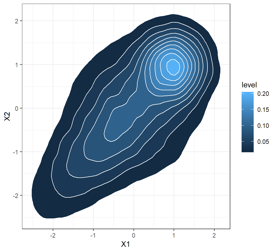
Gaussian mixture: K=3,p=2

Visualization of the Gaussian mixture:

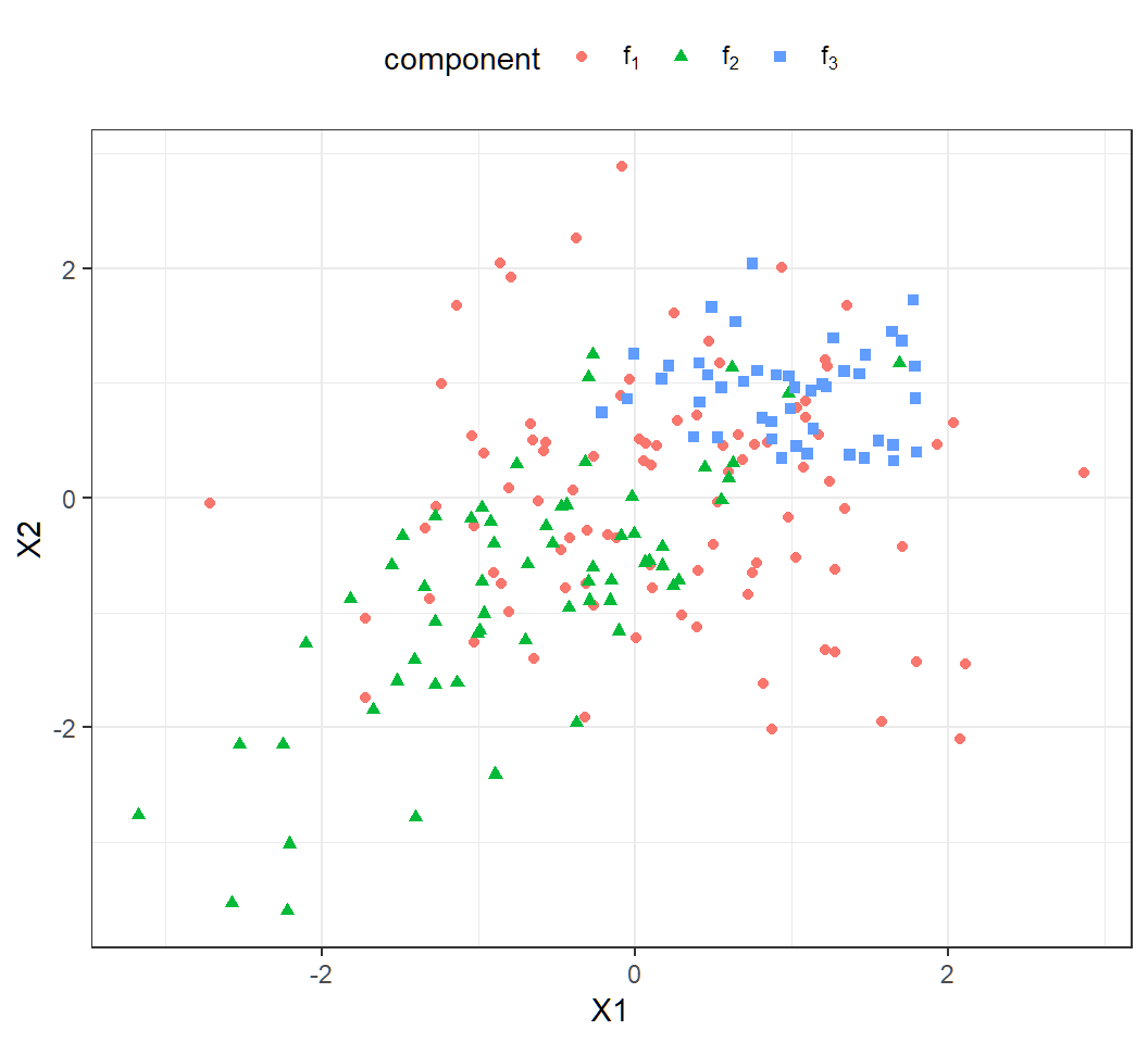
Gaussian mixture: K=3,p=2

\(n=200\) observations from the Gaussian mixture:

License and session Information

License

> sessionInfo()
R version 3.5.0 (2018-04-23)
Platform: x86_64-w64-mingw32/x64 (64-bit)
Running under: Windows 10 x64 (build 19041)

Matrix products: default

locale:
[1] LC_COLLATE=English_United States.1252 
[2] LC_CTYPE=English_United States.1252   
[3] LC_MONETARY=English_United States.1252
[4] LC_NUMERIC=C                          
[5] LC_TIME=English_United States.1252    

attached base packages:
[1] stats     graphics  grDevices utils     datasets  methods  
[7] base     

other attached packages:
[1] knitr_1.21

loaded via a namespace (and not attached):
 [1] compiler_3.5.0  magrittr_1.5    tools_3.5.0    
 [4] htmltools_0.3.6 revealjs_0.9    yaml_2.2.0     
 [7] Rcpp_1.0.0      stringi_1.2.4   rmarkdown_1.11 
[10] stringr_1.3.1   xfun_0.4        digest_0.6.18  
[13] evaluate_0.12