Discriminant function

Recall the log-posterior for \(X=x\) in Class \(k\) as \[ \begin{aligned} \log q_k(x) & =-\log\left[ \left( 2\pi\right) ^{p/2}\left\vert \Sigma_{k}\right\vert ^{1/2}\right] +\log\pi_{k}-\log f\left( x\right) \\ & -\frac{1}{2}x^{T}\Sigma_{k}^{-1}x+x^{T}\Sigma_{k}^{-1}\mu_{k}-\frac{1}{2}\mu_{k}^{T}\Sigma_{k}^{-1}\mu_{k} \end{aligned} \]

• If all \(\Sigma_{k}=\Sigma\), then the Class \(g\) that maximizes \(\log q_k(x),k\in\mathcal{G}\) also maximizes \[ \delta_k(x) = x^{T}\Sigma^{-1}\mu_{k}-\frac{1}{2}\mu_{k}^{T}\Sigma^{-1}\mu_{k} + \log\pi_{k}, k\in\mathcal{G}. \] So, \(\delta_k(x)\) is called a discriminant function
• Bayes classifier: \(X=x_0\) is classified into Class \(g\) if \(\delta_g(x_0)\) is the largest among all \(\delta_k(x_0),k\in\mathcal{G}\)

Linear discriminant function

• If all \(\Sigma_{k}=\Sigma\), the discriminant function \(\delta_k(x)\) is a linear function in \(x\), the “feature variables”, and is thus called linear discriminant function

• Further, when there is only \(p=1\) feature, then \(\mu_k\) is a scalar, \(\Sigma_{k}=\sigma^2\), \(\Sigma_{k}^{-1} =\sigma^{-2}\), and \(\delta_k(x)\) becomes \[ \delta_k(x) = x \frac{\mu_k}{\sigma^{2}} - \frac{\mu_k^2}{2\sigma^{2}} + \log\pi_{k} \]

• Linear discriminant analysis (LDA) uses an estimate \(\hat{\delta}_k(x)\) of \(\delta_k(x)\) to approximate the Bayes classifier when all \(\Sigma_{k}=\Sigma\)

LDA: pairwise decision boundary

• For \(k,l \in \mathcal{G}\) \[ \begin{aligned} D_{k,l}(x) & = \log \left(\frac{q_k(x)}{q_l(x)} \right) = \delta_k(x)-\delta_l(x)\\ & = \log\frac{\pi_{k}}{\pi_{l}}-\frac{1}{2}\left( \mu_{k}+\mu_{l}\right)^T\Sigma^{-1}\left(\mu_{k}-\mu_{l}\right)\\ & \quad +x^{T}\Sigma^{-1}\left( \mu_{k}-\mu_{l}\right) \end{aligned} \]

• So, \(\delta_k(x)=\delta_l(x)\) iff (if and only if) \(D_{k,l}(x)=0\), i.e., the decision boundary between Class \(k\) and Class \(l\) is the solution set \[ B_{k,l}=\{x \in \mathbb{R}^p: D_{k,l}(x)=0\}, \] which is a hyperplane in \(\mathbb{R}^p\)

LDA: pairwise decision boundary

Explanation on why \(B_{k,l}\) is a hyperplane:

• In the expression for \(D_{k,l}(x)\), we can write \[ \log\frac{\pi_{k}}{\pi_{l}}-\frac{1}{2}\left( \mu_{k} +\mu_{l}\right)\Sigma^{-1}\left( \mu_{k}-\mu_{l}\right) = b_{k,l} \in \mathbb{R} \] and \(\Sigma^{-1}\left( \mu_{k}-\mu_{l}\right)=\mathbf{c}_{k,l} \in \mathbb{R}^p\), which gives \[D_{k,l}(x)=b_{k,l}+x^{T}\mathbf{c}_{k,l}\]

• So, the solution \(x\) to \(D_{k,l}(x)=0\) is by definition a hyperplane in \(\mathbb{R}^p\)

• When \(p=1\), the solution is \(x=-b_{k,l}/\mathbf{c}_{k,l}\) if \(\mathbf{c}_{k,l} \ne 0\)

LDA: “plug-in” implementation

In practice, none of the \(\pi_{k}\)’s, \(\mu_{k}\)’s and \(\Sigma\) is known, and they need to be estimated. In the following, the hat \(\hat{}\) over a symbol denotes an estimate of the symbol.

• Training set \(\mathcal{T}=\{(x_i,y_i):i=1,\ldots,n\}\); let \(n_k\) be the number of observations in Class \(k\)
• MLEs: \(\hat{\pi}_{k}=n_{k}/n\), \(\hat{\mu}_{k}=\sum_{\left\{i:y_{i}=k\right\} }x_{i}/n_{k}\) and \[ \hat{\Sigma}=\frac{1}{n-K}\sum_{k=1}^{K}\sum_{\left\{ i:y_{i}=k\right\} }\left( x_{i}-\hat{\mu}_{k}\right) \left( x_{i}-\hat{\mu}_{k}\right) ^{T} \]
• Plug the estimates into \(\delta_{k}\) to get the estimate \(\hat{\delta}_{k}\) and apply LDA based on \(\hat{\delta}_{k}\)

LDA: “plug-in” implementation

• The MLE \(\hat{\Sigma}\) (given in previous slide) is the pooled covariance matrix estimate of \(\Sigma\)
• In general, for a \(\Sigma_k\), the sample covariance matrix \[ \hat{\Sigma}_k = \frac{1}{n_k-1}\sum_{\left\{ i:y_{i}=k\right\} }\left( x_{i}-\hat{\mu}_{k}\right) \left( x_{i}-\hat{\mu}_{k}\right) ^{T} \] is the MLE for \(\Sigma_k\)
• So, \(\hat{\Sigma}\) can be written as \[ \hat{\Sigma} = \frac{1}{n-K}\sum_{k=1}^{K} (n_k-1) \hat{\Sigma}_k \]

LDA: “plug-in” implementation

For LDA, the \(K\) component Gaussian densities have mean vectors \(\mu_k\) and a common covariance matrix \(\Sigma\).

• When there are \(p\) features, there are \((K-1)\times (p+1)\) parameters to estimate, since there \(K-1\) differences \(\delta_k(x)-\delta_K(x)\) and each difference has \(p+1\) parameters
• The MLEs of \(\mu_k\) and \(\Sigma\) usually work well when \(p\) is smaller than the sample size \(n\). But when \(p >n\), they are usually not accurate and the plug-in \(\hat{\delta}_{k}\) does not perform well for classification
• When \(p >n\), other estimates of \(\mu_k\) and \(\Sigma\) (such as regularized ones) are recommended

LDA: implementation

Regardless of the relative magnitudes of \(p\) and \(n\), we need to estimate \(K\), the number of classes, since \(K\) is unknown.

• \(K\) can be chosen by the Akaike information criterion (AIC) or Bayesian information criterion (BIC), which balances the predicitive performance of the Gaussian mixture model and its complexity

• Here “model complexity” takes into account \(K\) (roughly in the sense that the more parameters a model has, the more complicated it is)

LDA: Example 1 (K=2,p=1)

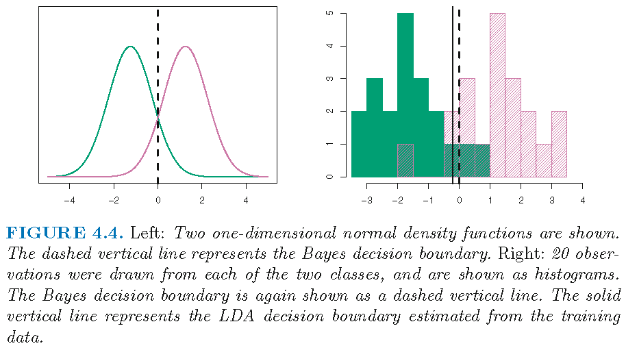
Consider the \(2\)-group Gaussian mixture with \[ \pi_1=\pi_2=0.5, \quad \mu_1 \ne \mu_2, \quad \sigma_1^2=\sigma_2^2=1 \] Then \[\delta_k(x) = x \mu_k - \mu_k^2/2 + \log\pi_{k}\]

• the decision boundary \(B_{1,2}\), as the solution to \(\delta_1(x)-\delta_2(x)=0\), contains the single point \[x=(\mu_1+\mu_2)/2,\] which is \(0\) if \(\mu_1=-\mu_2\)
• \(X=x\) is assigned to Class 1 if \(x\) satisfies \[ 2x \left( \mu_{1}-\mu_{2}\right) > \mu_{1}^2-\mu_{2}^2 \]

LDA: Example 1 (K=2,p=1)

• True decision boundary: \(x=(\mu_1+\mu_2)/2\)
• Estimated decision boundary is determined by \[ \hat{\delta}_1(x) = \hat{\delta}_2(x) \] where \[ \hat{\delta}_k(x) = x \frac{\hat{\mu}_k}{\hat{\sigma}^{2}} - \frac{\hat{\mu}_k^2}{2\hat{\sigma}^{2}} + \log \hat{\pi}_{k} \]
• With 40 observations such that \(n_1=n_2=20\), we have \(\hat{\pi}_{1}=\hat{\pi}_{2}=0.5\) and the estimated decision boundary as the single point \[x=(\hat{\mu}_1+\hat{\mu}_2)/2\]

LDA: Example 1 (K=2,p=1)

Test error: Bayes classifier (10.6%), LDA (11.1%)

LDA: Example 2 (p=2)

When \(p=2\) and \(\Sigma_k=\Sigma\),

• the discriminant function is \[ \delta_k(x) = x^{T}\Sigma^{-1}\mu_{k}-\frac{1}{2}\mu_{k}^{T}\Sigma^{-1}\mu_{k} + \log\pi_{k}, k\in\mathcal{G}, \]
• the pairwise decision boundary is a hyperplane in \(\mathbb{R}^2\), which is a line

If further \(\pi_k = \pi_0\), the pairwise decision boundary for Class \(k\) and \(l\) is the solution set to

\[ \begin{aligned} \frac{1}{2}\left( \mu_{k}+\mu_{l}\right)^T\Sigma^{-1}\left(\mu_{k}-\mu_{l}\right) =x^{T}\Sigma^{-1}\left( \mu_{k}-\mu_{l}\right) \end{aligned} \]

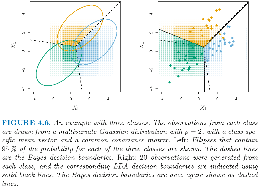
LDA: Example 2 (K=3,p=2)

Test error: Bayes classifier (0.0746), LDA (0.0770)

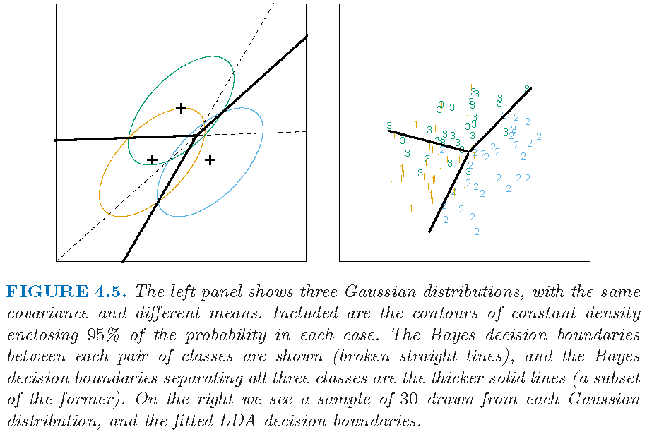
LDA: Example 3 (K=3,p=2)

Example from Supplementary Text:

Default data set

Default data set (in R library ISLR) on credit card users:

• 2 classes as statuses of default of a user on credit card payments, where default takes value Yes or No
  
• 3 features on each user: annual income, monthly credit card balance, user being student (with value Yes) or not (with value No)
• \(n=10,000\) training observations: 333 observations are for default=Yes, and the rest default=No

Target: apply LDA to classify a user’s status of default using some of the features

Default status and features

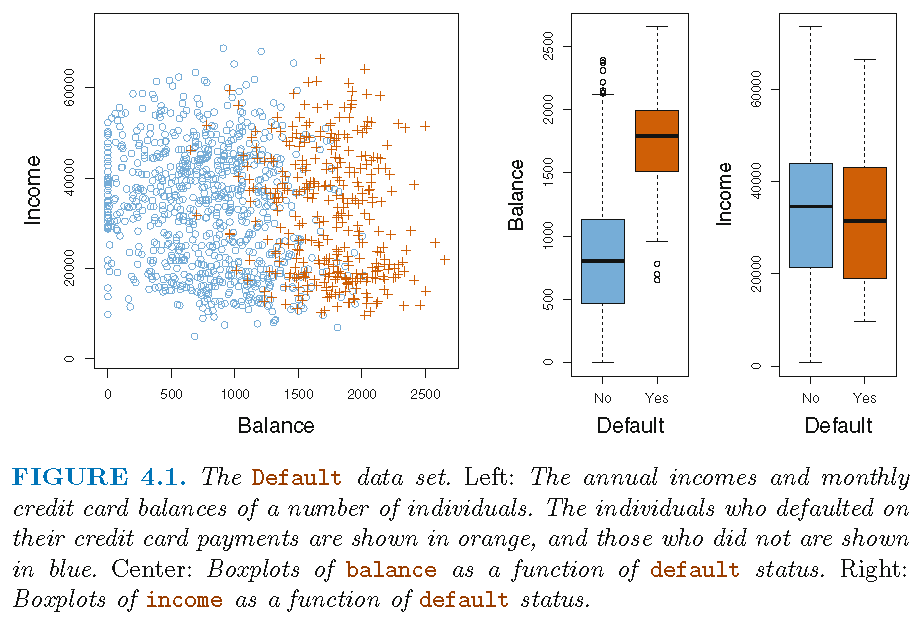Note: not all 10,000 observations are shown in the left panel

LDA applied to training set

LDA with features balance and student:

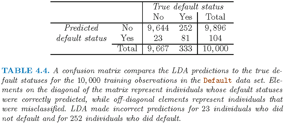
Verification of Table 4.4

A verification on Table 4.4, by applying LDA with features balance and student to training set:

                        TrueDefaultStatus
LDAEstimtedDefaultStatus   No  Yes
                     No  9644  252
                     Yes   23   81

• LDA requires observations on feature variables in each class to follow a Gaussian distribution
• It is insensible to apply LDA with student as a feature variable, unless the two values student=Yes and student=No are taken numerically and approximated by two Gaussian distributions with very small variances (that are close to \(0\)), respectively

LDA on training set

                        TrueDefaultStatus
LDAEstimtedDefaultStatus   No  Yes
                     No  9644  252
                     Yes   23   81

• LDA has a low training error of \(2.75\%=(252+23)/10^4\) based on \(n=10^4\) training samples. However, we are interested in test error
• Since only \(3.33\%=333/10^4\) of users in training sample defaulted (and training error approximates well test error under some conditions), the trivial null classifier (simple but useless) that always predicts default=No for a user will achieve an error rate that is only a bit higher than the LDA training error

Overall error and classwise error

                        TrueDefaultStatus
LDAEstimtedDefaultStatus   No  Yes
                     No  9644  252
                     Yes   23   81

• LDA predicted a total of 104 defaulters. Among them, only 23 out of the 9,667 non-defaulters were incorrectly identified. So, LDA has a very low error rate on the “non-defaulter class”
• Among the 333 defaulters, LDA missed 252; to identify high-risk users, an error rate of \(252/333 \approx 75.7\%\) on the “defaulter class” may well be unacceptable

Summary: on the training set, LDA has a low overall error rate but very high error rate on the defaulter class

Sensitivity and specificity

                        TrueDefaultStatus
LDAEstimtedDefaultStatus   No  Yes
                     No  9644  252
                     Yes   23   81

On the training set, LDA has

• sensitivity, here as “percentage of true defaulters that are identified”, \(81/333 \approx 24.3\%\)
• specificity, here as “percentage of non-defaulters that are correctly identified”, \(9644/9667 \approx 99.8\%\)

Note: sensitivity and specificity are measures on correct classifications

Why such performance?

Some reasons for LDA’s poor performance on training set:

• Model assumptions are probably violated
• Data set is dominated by observations in one class
• Not enough “telling” features are included in the model, i.e., credit card balance and student status probably are not features that are able to distinguish well defaulters from non-defaulters

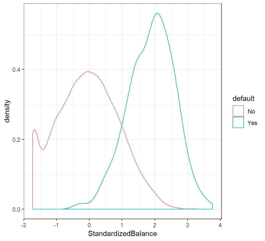
Non-Gaussian classwise feature

Classwise density of standardized balance:

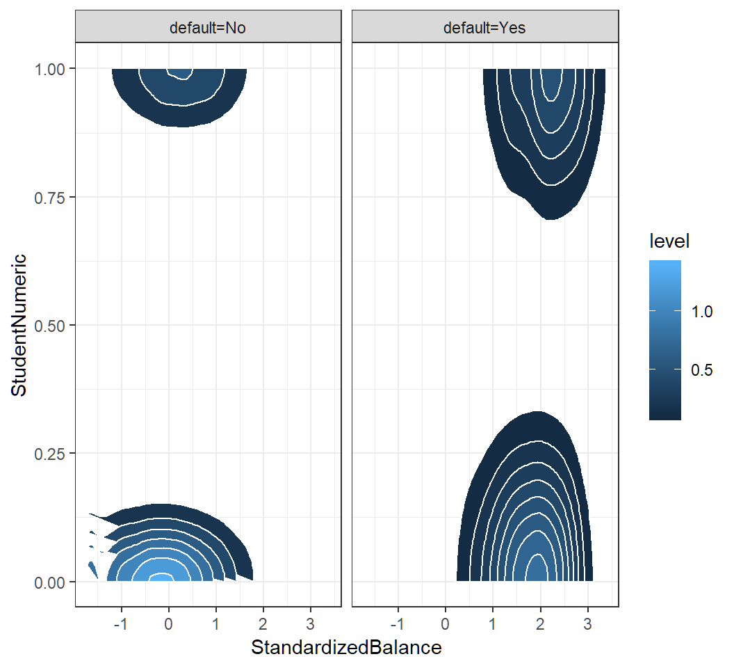
Non-Gaussian classwise features

student status: “No”\(\mapsto 0\) and “Yes”\(\mapsto 1\); values \(0\) and \(1\) are used as Gaussian means in component densities

Standard decision rule

• Bayes classifier uses the 0.5-treshold rule, i.e., it assigns Yes to a user’s default status if \[ q_1(x)=\Pr(\text{default}=\text{Yes}|X=x)>0.5, \] where \(X\) is the feature vector

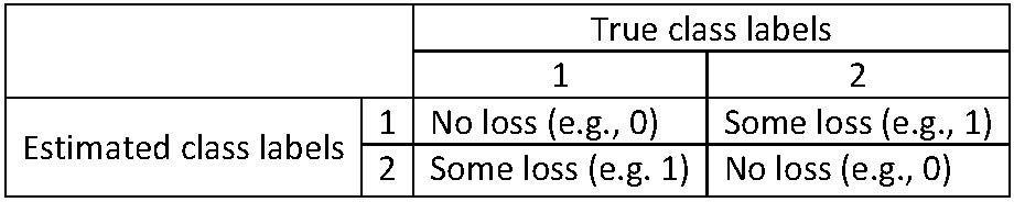
• LDA uses an estimate \(\hat{q}_1\) of \(q_1\), assigns Yes to a user’s default status if \(\hat{q}_1(x)>0.5\), and approximates Bayes classifier

• The 0-1 loss assigns equal weights to both types of missclassification, and the Bayes classifier minimizes the expected 0-1 loss

The 0-1 loss

Equal weights on both types of misclassification:

Modifying decision rule

• When classifying a non-defaulter as defaulter is less problematic than classifying a defaulter as a non-defaulter, assigning equal weights to both misclassification results, as done by the 0-1 loss, may be inappropriate

• If we are concerned about predicting the default status of a defaulter, then we can use a lower threshold, e.g., \(0.2\) instead of \(0.5\). Namely, a user’s default status is set as Yes if \[ q_1(x)=\Pr(\text{default}=\text{Yes}|X=x)>0.2 \]

• However, using a threshold different than 0.5 is equivalent to not using the Bayes classifier under the 0-1 loss

Modified decision rule: results

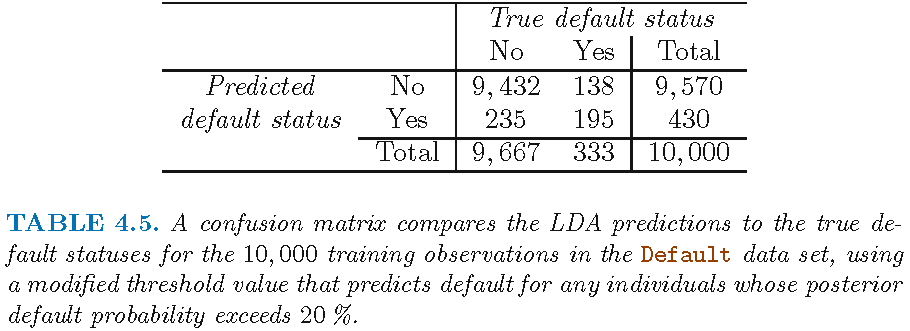
Modified LDA: results

LDA with features balance and student, applied to training set but with modified decision rule via \[\hat{q}_1(x)=\widehat{\Pr}(\text{default}=\text{Yes}|X=x)>0.2\]

                         TrueDefaultStatus
mLDAEstimtedDefaultStatus   No  Yes
                      No  9432  138
                      Yes  235  195

• overall error rate \(3.73\%=(138+235)/10^4\)
• error rate on defaulters: \(138/333 \approx 41.4\%\)
• error rate on non-defaulters: \(235/9667 \approx 2.4\%\)

Comparison of results

LDA with posterior threshold 0.5: overall error rate 2.75%; error rate on defaulters 75.7%

                        TrueDefaultStatus
LDAEstimtedDefaultStatus   No  Yes
                     No  9644  252
                     Yes   23   81

LDA with posterior threshold 0.2: overall error rate 3.73%; error rate on defaulters 41.4%

                         TrueDefaultStatus
mLDAEstimtedDefaultStatus   No  Yes
                      No  9432  138
                      Yes  235  195

Profile of modified decision rule

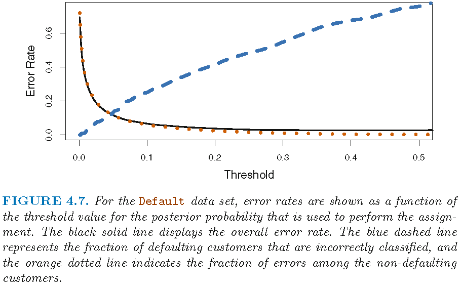
Profile of modified decision rule

• Threshold value 0.5 minimizes overall error rate, since the Bayes classifier uses this value and has the lowest overall error rate (when models are specified correctly, which for LDA is the Gaussian mixture model). However, this value gives high error rate on the defaulter class

• A the threshold is reduced, error rate on the defaulter class decreases but error rate on the non-defaulters class increases

• Domain knowledge is needed to determine which threshold value to use

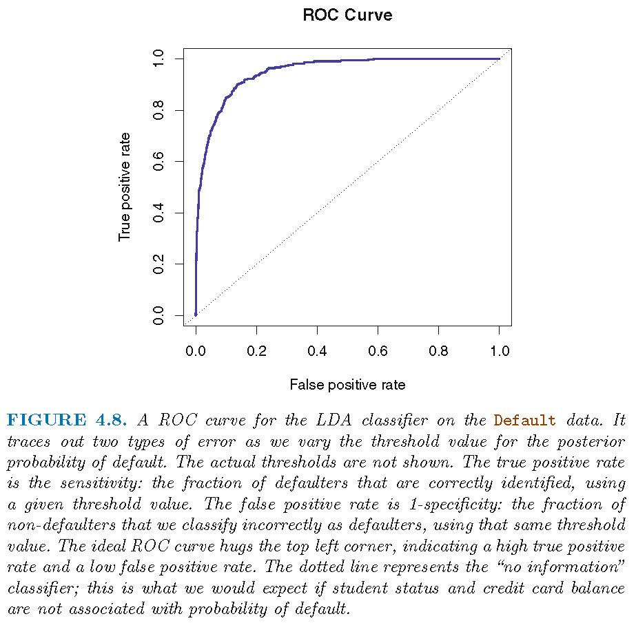
ROC and AUC

• The receiver operating characteristics (ROC) curve is a popular graphic for simultaneously displaying the two types of errors for all possible thresholds
• ROC curves are useful for comparing different classifiers, since they take into account all possible thresholds
• The overall performance of a classifier, summarized over all possible thresholds, is given by the area under the (ROC) curve (AUC)
• We expect a classifier that performs no better than chance to have an AUC of 0.5 (when evaluated on an independent test set not used in model training)

ROC and AUC

The AUC is 0.95 for this data set:

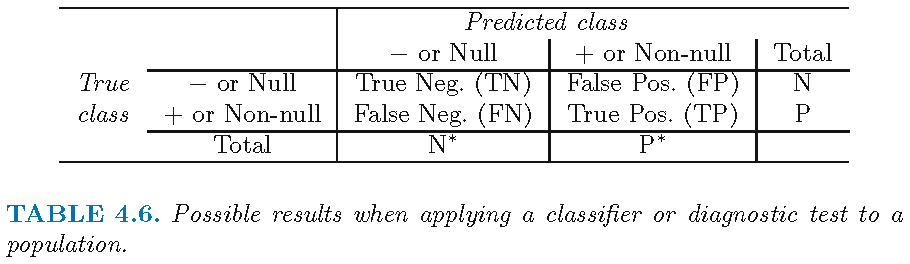
Terms on error types

In the example: “default=Yes” \(\mapsto +\); “default=No” \(\mapsto -\)

Discriminant function

Recall the log-posterior for \(X=x\) in Class \(k\) as \[ \begin{aligned} \log q_k(x) & =-\log\left[ \left( 2\pi\right) ^{p/2}\left\vert \Sigma_{k}\right\vert ^{1/2}\right] +\log\pi_{k}-\log f\left( x\right) \\ & -\frac{1}{2}x^{T}\Sigma_{k}^{-1}x+x^{T}\Sigma_{k}^{-1}\mu_{k}-\frac{1}{2}\mu_{k}^{T}\Sigma_{k}^{-1}\mu_{k} \end{aligned} \]

• When \(\Sigma_{k}\) are not equal, the Class \(g\) that maximizes \(\log q_k(x),k\in\mathcal{G}\) also maximizes for all \(k\in\mathcal{G}\) \[ \begin{aligned} \delta_{k}\left( x\right) & =-\frac{1}{2}\log\left\vert \Sigma_{k}\right\vert-\frac{1}{2}\mu_{k}^{T}\Sigma_{k}^{-1}\mu_{k}+\log\pi_{k}\\ & \quad -\frac{1}{2}x^{T}\Sigma_{k}^{-1}x+x^{T}\Sigma_{k}^{-1}\mu_{k} \end{aligned} \]

Quadratic discriminant function

• Bayes classifier: \(X=x_0\) is classified into Class \(g\) if \(\delta_g(x_0)\) is the largest among all \(\delta_k(x_0),k\in\mathcal{G}\)
• The term “\(-\frac{1}{2}x^{T}\Sigma_{k}^{-1}x\)” in \(\delta_{k}\left( x\right)\) indicates that \(\delta_{k}\left( x\right)\) is a quadratic function of \(x\), the “feature variables”
• Further, when there is only \(p=1\) feature, \(\mu_k\) is a scalar, \(\Sigma_{k}=\sigma_k^2\), \(\Sigma_{k}^{-1} =\sigma_k^{-2}\), and \(\delta_k(x)\) becomes \[ \delta_k(x) = - \frac{x^2}{2\sigma_k^2} +x \frac{\mu_k}{\sigma_k^{2}} - \frac{\mu_k^2}{2\sigma_k^{2}} -\log \sigma_k + \log\pi_{k} \]
• Quadratic discriminant analysis (QDA) uses an estimate \(\hat{\delta}_k\) of \(\delta_k\) to approximate the Bayes classifier when \(\Sigma_{k}\)’s are different

QDA: pairwise decision boundary

• When \(\Sigma_{k}\)’s are different, for \(k,l \in \mathcal{G}\) \[ \begin{aligned} D_{k,l}(x) & = \log \left[{q_k(x) }/{q_l(x) } \right] = \delta_k(x)-\delta_l(x)\\ & =\log\frac{\pi_{k}}{\pi_{l}}- \frac{1}{2}\log \frac{\vert \Sigma_k\vert}{\vert \Sigma_l\vert} -\frac{1}{2}\left(x-\mu_{k}\right)^T\Sigma_k^{-1}\left(x-\mu_{k}\right) \\ & \quad +\frac{1}{2}\left(x-\mu_{l}\right)^T\Sigma_l^{-1}\left(x-\mu_{l}\right) \end{aligned} \]

• So, \(\delta_k(x)=\delta_l(x)\) iff \(D_{k,l}(x)=0\), i.e., the decision boundary between Class \(k\) and Class \(l\) is the solution set \[ B_{k,l}=\{x \in \mathbb{R}^p: D_{k,l}(x)=0\}, \] which is NOT a hyperplane in \(\mathbb{R}^p\) when \(\Sigma_{k}\)’s are different

QDA: pairwise decision boundary

Explanation on why \(B_{k,l}\) is not a hyperplane:

• \(D_{k,l}(x)\) can be written as \[ D_{k,l}(x) = 2^{-1} x^T A_{k,l}x+ x^T \mathbf{c}_{k,l}+b_{k,l} \] with \(A_{k,l}=\Sigma_l^{-1}-\Sigma_k^{-1}\) (a \(p\times p\) matrix), \(b_{k,l} \in \mathbb{R}\), and \(\mathbf{c}_{k,l}=\Sigma_k^{-1} \mu_k - \Sigma_l^{-1} \mu_l \in \mathbb{R}^p\)
  
• So, the solution \(x\) to \(D_{k,l}(x)=0\) is not a hyperplane in \(\mathbb{R}^p\) if \(A_{k,l} \ne 0\)
• When \(p=1\), \(\Sigma_k=\sigma_k^2\) and the solution, if \(\sigma_k^2 \ne \sigma_l^2\), is \[ x=\frac{-\mathbf{c}_{k,l} \pm \sqrt{\mathbf{c}_{k,l}^2 -2 (\sigma_l^{-2}-\sigma_k^{-2})b_{k,l}}}{\sigma_l^{-2}-\sigma_k^{-2}} \]

QDA: “plug-in” implementation

In practice, none of the \(\pi_{k}\)’s, \(\mu_{k}\)’s and \(\Sigma_k\)’s are known, and they need to be estimated.

• Training set \(\mathcal{T}=\{(x_i,y_i):i=1,\ldots,n\}\); let \(n_k\) be the number of observations in Class \(k\)
• MLEs: \(\hat{\pi}_{k}=n_{k}/n\), \(\hat{\mu}_{k}=\sum_{\left\{i:y_{i}=k\right\} }x_{i}/n_{k}\) and \[ \hat{\Sigma}_k = \frac{1}{n_k-1}\sum_{\left\{ i:y_{i}=k\right\} }\left( x_{i}-\hat{\mu}_{k}\right) \left( x_{i}-\hat{\mu}_{k}\right) ^{T} \]
• Plug the estimates into \(\delta_{k}\) to get the estimate \(\hat{\delta}_{k}\) and apply QDA based on \(\hat{\delta}_{k}\)

QDA: “plug-in” implementation

For QDA, the \(K\) component Gaussian densities have mean vectors \(\mu_k\) and covariance matrices \(\Sigma_k\).

• When there are \(p\) features, there are \((K-1)\times \left[p(p+3)/2+1\right]\) parameters to estimate, since there are \(K-1\) differences \(\delta_k(x)-\delta_K(x)\) and each difference has respectively \(p(p+1)/2\), \(p\) and \(1\) parameters for its quadratic, linear and 0th order term

• The MLEs of \(\mu_k\) and \(\Sigma_k\) usually work well when \(p\) is smaller than the sample size \(n\). But when \(p >n\), they are usually not accurate and the plug-in \(\hat{\delta}_{k}\) may not perform well in classification

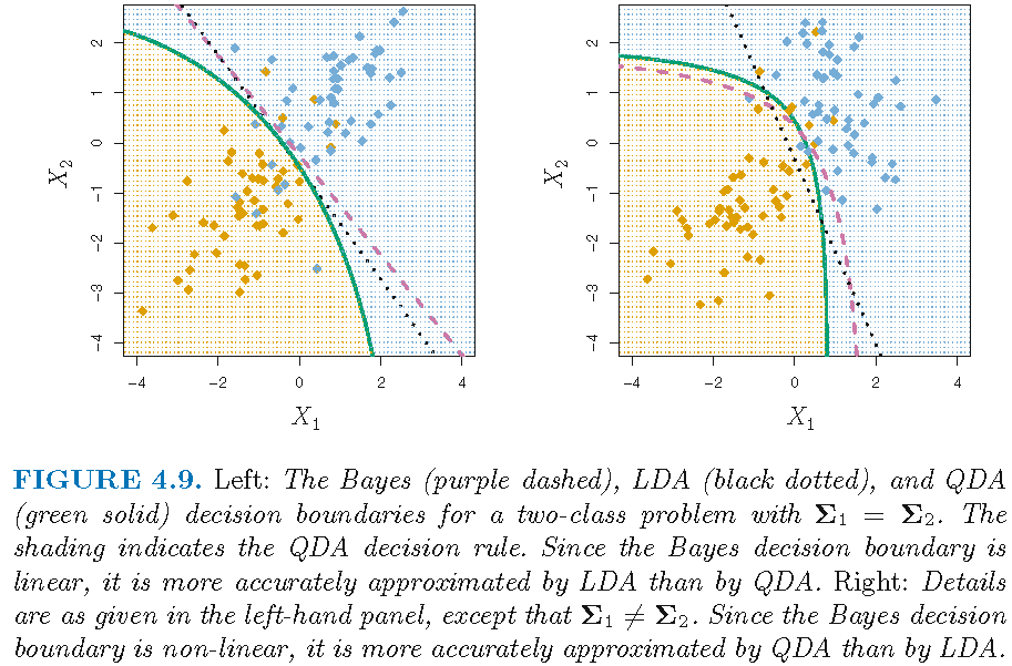
LDA versus QDA

• LDA and QDA both employ a Gaussian mixture model
• LDA assumes equal component covariance matrices, and QDA does not. So, LDA is less flexible (i.e., has larger bias) and more stable (i.e., has smaller variance) than QDA
• LDA tends to be a better choice than QDA if there are relatively few training observations and so reducing variance is crucial, whereas QDA is recommended if training set is very large, so that variance of the classifier is not a major concern, or if assumption of a common covariance matrix is clearly untenable
• Neither may work well if mis-applied

LDA versus QDA

Choice of LDA or QDA depends on data:

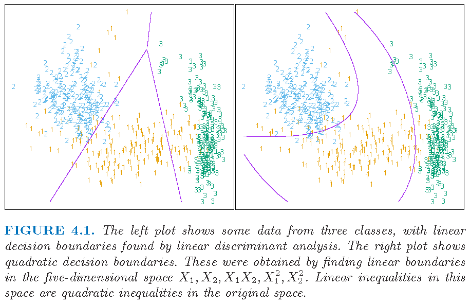
LDA on transformed features

LDA on transformed feature variables:

• Original 2 feature variables \(X_1\) and \(X_2\), giving a 2-dimensional feature space
• 5 transformed feature variables: \(X_{1},X_{2},X_{1}X_{2},X_{1}^{2}\) and \(X_{2}^{2}\), which are functionally linearly independent but not statistically independent, giving a 5-dimensional feature space

Caution: LDA with original feature variables has linear decision boundary in original feature space. However, LDA with nonlinearly transformed feature variables has nonlinear decision boundary in original feature space.

LDA on transformed features

Explanation on functional/statistical independence:

• The polynomials \(X_{1},X_{2},X_{1}X_{2},X_{1}^{2}\) and \(X_{2}^{2}\) are functionally linearly independent, i.e., if there are constants \(\left\{ a_{i}\right\}_{i=1}^{5}\) such that \[ a_{1}X_{1}+a_{2}X_{2}+a_{3}X_{1}X_{2}+a_{4}X_{1}^{2}+a_{5}X_{2}^{2}=0, \] then \(a_{i}=0\) for all \(i\)
• However, they are not statistically independent since, e.g., \(X_{2}^{2}\) is not probabilistically independent of \(X_{2}\), and \(X_{1}X_{2}\) is not probabilistically independent of either \(X_1\) or \(X_2\)
• The dimension of a linear space spanned by some functions is determined by functional linear independence

LDA on transformed features

Figure 4.1 from Supplementary Text:

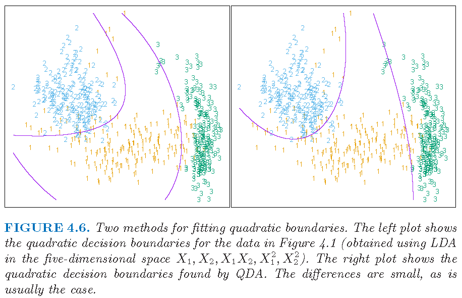
DA on transformed features

Figure 4.6 from Supplementary Text: LDA on transformed features may perform close to QDA on original features

Regularized DA

When \(p >n\), other estimates of \(\Sigma_k\) (different than the MLE) are recommended, such as

• regularized estimate: \[\hat{\Sigma}_{k,\alpha}=\alpha \hat{\Sigma}_k + (1-\alpha) \hat{\Sigma}, \alpha \in [0,1]\] where \(\hat{\Sigma}\) is a pooled covariance matrix (as used in LDA) and \(\hat{\Sigma}_k\) can be the sample covariance matrix of observations in Class \(k\), and further \(\hat{\Sigma}\) can be a shrinkage estimate as \[\hat{\Sigma}_{\gamma}= \gamma \hat{\Sigma} + (1-\gamma) \hat{\sigma}^2 \mathbf{I}, \gamma \in [0,1]\]
• Similar regularized or shrinkage estimates of \(\mu_k\) can also be used

Regularized DA

For the regularized estimate \[\hat{\Sigma}_{k,\alpha}=\alpha \hat{\Sigma}_k + (1-\alpha) \hat{\Sigma}, \alpha \in [0,1]\]

• \(\alpha \approx 1\) implies different \(\hat{\Sigma}_{k,\alpha}\)’s, and hence analysis is close to QDA
• \(\alpha \approx 0\) implies similar \(\hat{\Sigma}_{k,\alpha}\)’s, and hence analysis is close to LDA

DA with regularized or shrinkage estimates is called regularized discriminant analysis (RDA)

Note: contents on RDA adopted from Section 4.3.1 of Supplementary Text

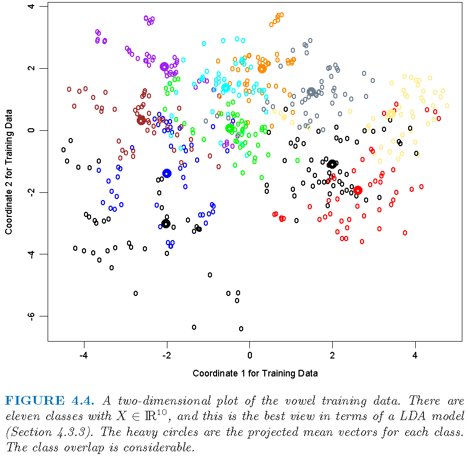
Regularized DA: vowel data

Figure 4.4 from Supplementary Text:

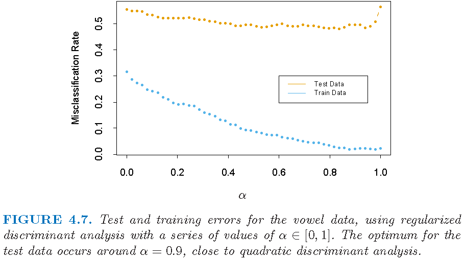
Regularized DA: error rates

Figure 4.7 from Supplementary Text:

QDA: Default data

Default data set (in R library ISLR) on credit card users:

• 2 classes as statuses of default of a user on credit card payments, where default takes value Yes or No
  
• 3 features on each user: annual income, monthly credit card balance, user being student (with value Yes) or not (with value No)
• \(n=10,000\) training observations: 333 observations are for default=Yes, and the rest default=No

Target: apply LDA to classify a user’s status of default using some of the features

QDA: Default data

Check Gaussian assumption: student hidden in contours

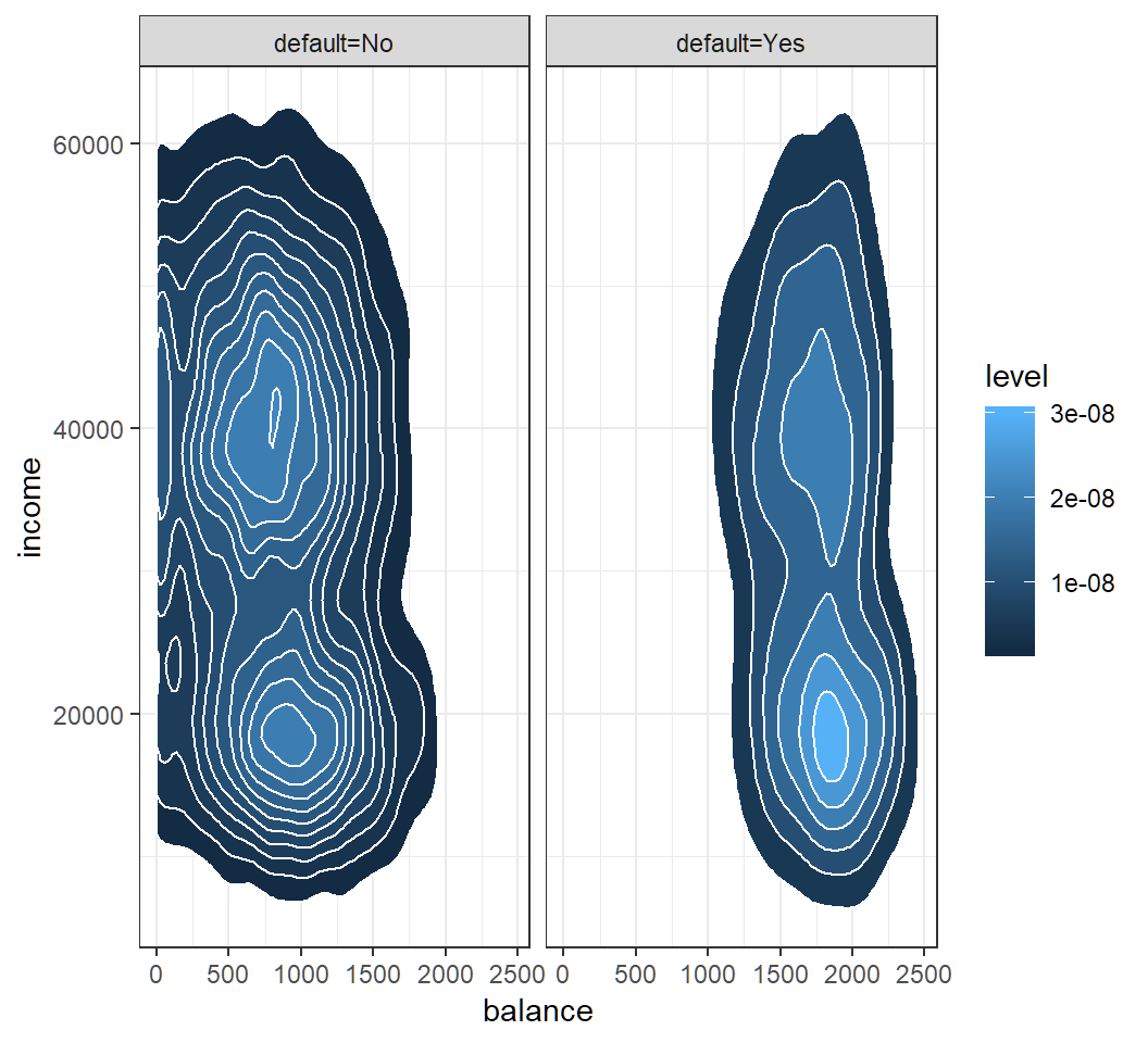
QDA: classification

Classification results of QDA with features balance and income on training set and “0.5-threshold rule” of default=Yes if \(\widehat{\Pr}(\text{default}=\text{Yes}|X=x)>0.5\):

                        TrueDefaultStatus
QDAEstimtedDefaultStatus   No  Yes
                     No  9637  241
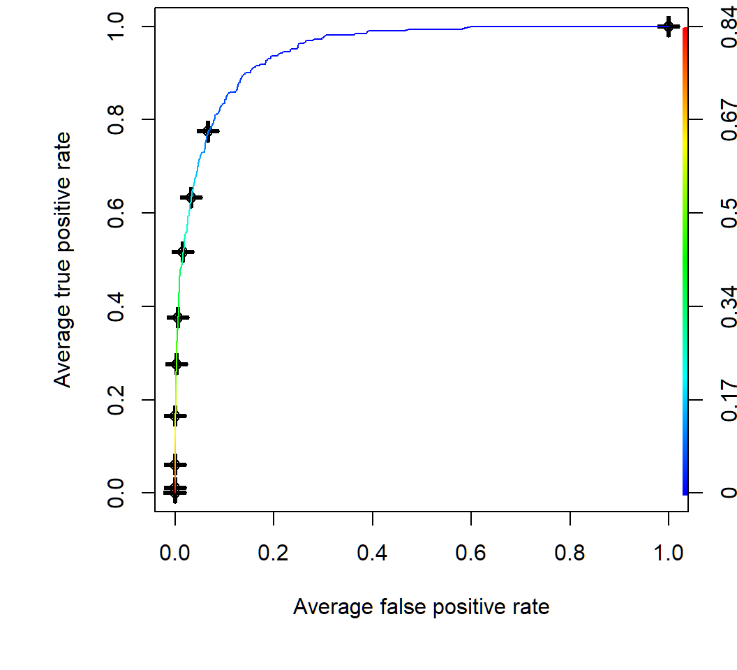
                     Yes   30   92

AUC:

[1] 0.9489247

Create ROC curves by CV

Average of 10 ROC curves obtained by 10-fold cross-validation; color key for threshold value on posterior of default class in R

Overall comparsion

• LDA and QDA are parametric and employ a Gaussian mixture model
• Logistic regression can outperform LDA or QDA if the assumption on a Gaussian mixture model is violated
• kNN method is non-parametric, and it can dominate LDA and logistic regression approaches when decision boundary is highly non-linear or complicated. However, kNN method does not tell us which predictors or features are important
• QDA is a compromise between kNN method, LDA and logistic regression

Logistic regression and LDA

Difference 1:

• Logistic regression does not employ a mixture model, and it takes \[q_k(x)=\Pr\left(Y=k|X=x\right)\] as the conditional probability of \(X=x\) when it is generated using Class \(k\) conditional density \(f_k\)

• LDA employs a Gaussian mixture model and takes \[q_k(x)=\Pr\left(Y=k|X=x\right)\] as the posterior probability of \(X=x\) in Class \(k\) after \(x\) is obtained

Logistic regression and LDA

• For LDA, we have \[ \log \left(\frac{q_k(x)}{q_K(x)}\right)=b_{k}+\mathbf{c}_{k}^{T}x, \quad k \in \{1,\ldots,K-1\}, \] where \(b_{k}\) and \(\mathbf{c}_{k}\) are functions of \(\mu_k,\mu_K,\pi_k,\pi_K,\Sigma_k\) and \(\Sigma_K\)
• For logistic regression, we have \[ \begin{aligned} \log \left(\frac{q_k(x)}{q_K(x)}\right) = \beta_{k0} + \boldsymbol{\alpha}_{k}^T x, \quad k \in \{1,\ldots,K-1\}, \end{aligned} \] where \(\boldsymbol{\alpha}_{k}=(\beta_{k1},\ldots,\beta_{kp})^T\) and \(\beta_{k0}\) are parameters

Similarity 1: both methods employ linear modelling equations for log-odds

Logistic regression and LDA

Recall \[ \begin{aligned} \Pr\left( Y=k|X=x\right)= \left[\Pr\left(Y=k\right)\Pr(X=x|Y=k)\right] \div {f(x)}, \end{aligned} \] where \(f\) is the marginal density of \(X\)

Difference 2:

• Logistic regression does not need the marginal distribution \(F\) of \(X\), and maximizes the conditional likelihood \(\Pr\left(Y=k|X\right)\) given observations from \(X\)

• LDA aims to obtain maximal posterior \(\Pr(Y=g|X)\) when it classifies \(X\) into Class \(g\) and hence implicitly uses \(F\) to maximize the joint likelihood on \((X,Y)\)

Logistic regression and LDA

Difference 3:

• If observations can be perfectly separately by a hyperplane into two classes, then for logistic regression the maximum likelihood estimates of the regression parameters are undefined (since logistic regression does not use the marginal distribution of feature variables)

• However, in this case, the LDA coefficients for the same data will be well defined and LDA can be implemented, since LDA uses the marginal distribution of feature variables and this marginal distribution will not permit such degeneracies in parameter estimation

Comparison: setup

• 2 features and 2 classes

• 100 random training data sets

• 6 methods: kNN-1, kNN-CV, LDA, Logistic regression, and QDA

• On each training set, fit each of 6 methods to the training data, and obtain the resulting test error on a large test set

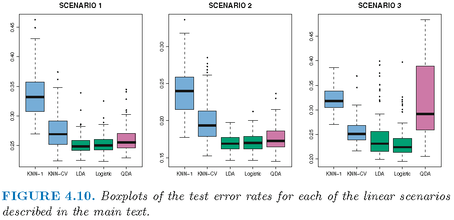
Setting for linear boundary

• Scenario 1: uncorrelated Gaussian feature variables, with 20 observations per class; LDA overall winner

• Scenario 2: equally correlated Gaussian feature variables across component bivariate Gaussian densities, with 20 observations per class; LDA overall winner

• Scenario 3: uncorrelated Student t feature variables with 50 observations per class, violating assumptions of LDA and QDA; logistic regression overall winner

Results: linear boundary

Winner: LDA (Scenario 1 and 2); Logistic (Scenario 3)

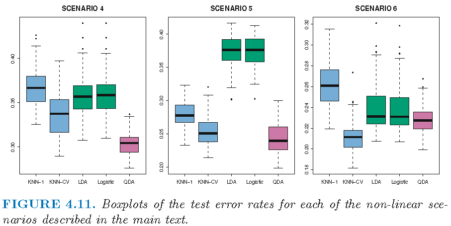
Setting for non-linear boundary

• Scenario 4: unequally correlated Gaussian feature variables across component bivariate Gaussian densities; QDA overall winner

• Scenario 5: uncorrelated Gaussian feature variables within each class but class labels sampled from the logistic function using squared features; QDA overall winner

• Scenario 6: as Scenario 5 but class labels sampled from a more complicated non-linear function of features; kNN-CV overall winner

Resuls: non-linear boundary

Winner: QDA (Scenario 4 and 5); kNN-CV (Scenario 6)

License and session Information

License

> sessionInfo()
R version 3.5.0 (2018-04-23)
Platform: x86_64-w64-mingw32/x64 (64-bit)
Running under: Windows 10 x64 (build 19041)

Matrix products: default

locale:
[1] LC_COLLATE=English_United States.1252 
[2] LC_CTYPE=English_United States.1252   
[3] LC_MONETARY=English_United States.1252
[4] LC_NUMERIC=C                          
[5] LC_TIME=English_United States.1252    

attached base packages:
[1] stats     graphics  grDevices utils     datasets  methods  
[7] base     

other attached packages:
[1] knitr_1.21

loaded via a namespace (and not attached):
 [1] compiler_3.5.0  magrittr_1.5    tools_3.5.0    
 [4] htmltools_0.3.6 revealjs_0.9    yaml_2.2.0     
 [7] Rcpp_1.0.0      stringi_1.2.4   rmarkdown_1.11 
[10] stringr_1.3.1   xfun_0.4        digest_0.6.18  
[13] evaluate_0.12