Stat 437 Lecture Notes 5c

Xiongzhi Chen

Washington State University

Discriminant analysis: Example 3

Human cancer microarray data

Human cancer microarray data:

6830 genes (i.e., 6830 features)
64 samples (i.e., 64 cancer cell lines)
14 different cancer types; information on cancer types at wiki-NCI60

The data matrix has dimension $6830 \times 64$, each of whose columns is an observation for all features.

We will pick 3 caner types “BREAST”, “LEUKEMIA” and “COLON”, and randomly select the same set of $50$ genes for each cancer type

Obtain subset of data

> library(ElemStatLearn) # library containing data
> data(nci); n0=dim(nci)[2]; p0=dim(nci)[1] #get dimensions
> set.seed(123)
> rSel = sample(1:p0, size=50, replace = FALSE)
> chk = colnames(nci) %in% c("BREAST", "LEUKEMIA", "COLON")
> cSel = which(chk ==TRUE)
> ncia = nci[rSel,cSel]
> colnames(ncia) = colnames(nci)[cSel]

colnames(nci): each column name is the cancer type for an observation
chk: check if a cancer type is “BREAST”, “LEUKEMIA” or “COLON”
take features (i.e., genes) from rows of nci, and take samples (i.e., observations for features) from columns of nci

Glimpse on subset of data

> # transposed subset data as `tmp`
> tmp = data.frame(t(ncia)); tmp$Class=colnames(ncia)
> rownames(tmp)=NULL; dim(tmp)
[1] 20 51
> table(tmp$Class)

  BREAST    COLON LEUKEMIA 
       7        7        6 
> tmp[1:3,(ncol(tmp)-3):ncol(tmp)]
     X48    X49   X50  Class
1 -0.415 -0.735 1.935 BREAST
2 -0.040 -0.780 0.060 BREAST
3  0.750 -0.320 1.800 BREAST

the last entry of each row of tmp is the cancer type of an observation, and the rest in each such row is an observation on the features
$p=50$ feature variables $X_1,\ldots,X_{50}$, and $n=20$ observations; $p > 2n$

Visualize subset of data

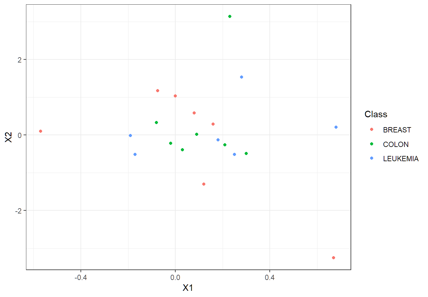
In terms of class memberships, observations overlap each other much?

Visualize subset of data

Each observation on the $p=50$ features (is in $\mathbb{R}^{50}$ and) is a 50-dimensional vector.

When such observations are visualized via only 2 features, to our eyes they may overlap each other in terms of class memberships. Namely, visualization of vectors in much lower dimensions may show overlap among these vectors.
However, when viewed in their ambient space $\mathbb{R}^{p}$, they may not overlap at all (since neighborhoods of a vector are different in spaces of different dimensions).
Think about an overpass on a highway, which “intersects” the highway when both are viewed from above (equivalent to visualizing them in 2D)

LDA: p > 2n

LDA with 50 feature variables, 3 classes, and sample size 20:

> library(MASS)
> lda.fit = lda(Class~.,data=tmp)
Warning in lda.default(x, grouping, ...): variables are
collinear
> lda.pred = predict(lda.fit,tmp)
> TrueClassLabel=tmp$Class
> LDAEstimtedClassLabel=lda.pred$class
> table(LDAEstimtedClassLabel,TrueClassLabel)
                     TrueClassLabel
LDAEstimtedClassLabel BREAST COLON LEUKEMIA
             BREAST        6     0        0
             COLON         1     7        0
             LEUKEMIA      0     0        6

Classwise error rates: “BREAST”, “LEUKEMIA” and “COLON”

[1] 0.1428571 0.0000000 0.0000000

Standard estimates of covariance matrix are singular!!

QDA: p > 2n

The component covariance matrices may not be equal since gene profiles for different cancer types may have different dependence structures. So, let us apply QDA:

> library(MASS)
> qda.fit = qda(Class~.,data=tmp)
> # Error in qda.default(x, grouping, ...) : 
> #   some group is too small for 'qda'

Not enough observations in each group to sensibly estimate the corresponding component parameters
Standard estimates of component covariance matrices are singular!!

Singular DA: p > n

LDA: pooled covariance matrix estimate \[ \hat{\Sigma}=\frac{1}{n-K}\sum_{k=1}^{K}\sum_{\left\{ i:y_{i}=k\right\} }\left( x_{i}-\hat{\mu}_{k}\right) \left( x_{i}-\hat{\mu}_{k}\right) ^{T} \] as an estimate of $\Sigma$
QDA: sample covariance matrix \[ \hat{\Sigma}_k = \frac{1}{n_k-1}\sum_{\left\{ i:y_{i}=k\right\} }\left( x_{i}-\hat{\mu}_{k}\right) \left( x_{i}-\hat{\mu}_{k}\right) ^{T} \] as an estimate of $\Sigma_k$

Caution: when $p >n$, $\hat{\Sigma}$ and all $\hat{\Sigma}_k$ are all singular, not being valid covariance matrices or forcing some feature variables to be linearly dependent!

Regularized DA

When $p >n$, we can use the regularized estimate proposed by “Friedman, J.H. (1989): Regularized Discriminant Analysis” and implemented by R library klaR.
The regularized estimate of $\Sigma_k$ is \[ \hat{\Sigma}_{k,\lambda,\gamma}= (1-\gamma) \hat{\Sigma}_{k,\lambda} + \gamma p^{-1} \text{tr}(\hat{\Sigma}_{k,\lambda}) \mathbf{I}, \gamma \in [0,1] \] with \[\hat{\Sigma}_{k,\lambda}=(1-\lambda) \hat{\Sigma}_k + \lambda \hat{\Sigma}, \lambda \in [0,1]\] where $\hat{\Sigma}$ is a pooled covariance matrix, $\hat{\Sigma}_k$ is a suitable estimate of $\Sigma_k$, and $\text{tr}(A)$ is the trace of the square matrix $A$, i.e., the sum of the diagonal entries of $A$

Regularized DA via `klaR`

We need R library klaR, and command rda{klaR} for which the basic syntax is

rda(formula, data, gamma = 0.05, lambda = 0.2,
     crossval = FALSE, ...)

formula: the same as in lda or qda
gamma, lambda: same as $\gamma$ and $\lambda$ in $\hat{\Sigma}_{k,\lambda,\gamma}$. If unspecified, either or both are determined by minimizing the estimated error rate
crossval: logical. If TRUE, then the error rate is estimated by Cross-Validation; otherwise, by drawing several training- and test-samples.

Regularized DA via `klaR`

rda{klaR} returns a list of class rda containing the following components:

regularization: vector containing the two regularization parameters (gamma, lambda).
classes and prior: the names of the classes, and the prior probabilities for the classes.
error.rate: apparent error rate (if computation was not suppressed), and, if any optimization took place, the final (cross-validated or bootstrapped) error rate estimate as well.

Regularized DA via `klaR`

rda{klaR} returns a list of class rda containing the following components:

means, covariances and covpooled: group means, array of group covariances, and pooled covariance.
converged: (Logical) indicator of convergence (only for Nelder-Mead).
iter: number of iterations actually performed (only for Nelder-Mead).

Regularized DA via `klaR`

RDA on the subset data ($p=50$ and $n=20$):

> library(klaR)
> rda.fit = rda(Class~.,data=tmp, gamma = 0.05, lambda = 0.2)
> rda.pred = predict(rda.fit, tmp) # classify obs in `tmp`
> TrueClassLabel=tmp$Class
> rDAEstimtedClassLabel=rda.pred$class
> table(rDAEstimtedClassLabel,TrueClassLabel)
                     TrueClassLabel
rDAEstimtedClassLabel BREAST COLON LEUKEMIA
             BREAST        7     0        0
             COLON         0     7        0
             LEUKEMIA      0     0        6

predict acts on an object of class rda similarly as MASS::predict on an object of class lda or qda
good results; not determining gamma or lambda via cross-validation due to n=20

Extract est. covariance matrices

> # extract estimated covariance matrices
> hatSigma1 = rda.fit$covariances[,,1]
> hatSigma2 = rda.fit$covariances[,,2]
> hatSigma3 = rda.fit$covariances[,,3]

rda(...)$covariances: a $p \times p \times K$ array. To obtain the estimated covariance matrix, $\hat{\Sigma}_{k,\lambda,\gamma}$, of observations in Class $k$, use rda(...)$covariances[,,k]. Note that class (and label) ordering is determined by rda using rules of R.

Melt est. covariance matrices

> # convert estimated covariance matrices for plotting 
> library(reshape2)
> melted_hatSigma1 = melt(hatSigma1)
> melted_hatSigma2 = melt(hatSigma2)
> melted_hatSigma3 = melt(hatSigma3)
> EstSigmaAll=rbind(melted_hatSigma1,melted_hatSigma2,
+                   melted_hatSigma3)
> EstSigmaAll$Cancer=rep(c("BREAST","COLON","LEUKEMIA"),
+                          each=nrow(melted_hatSigma1))
> EstSigmaAll$Cancer=factor(EstSigmaAll$Cancer)

melt(data,value.name ="value",...): convert data into a molten data.frame, and by default store entries of data as "value" in the molten data.frame, as if values in data are values of a function that are obtained on a 2D grid on two variables

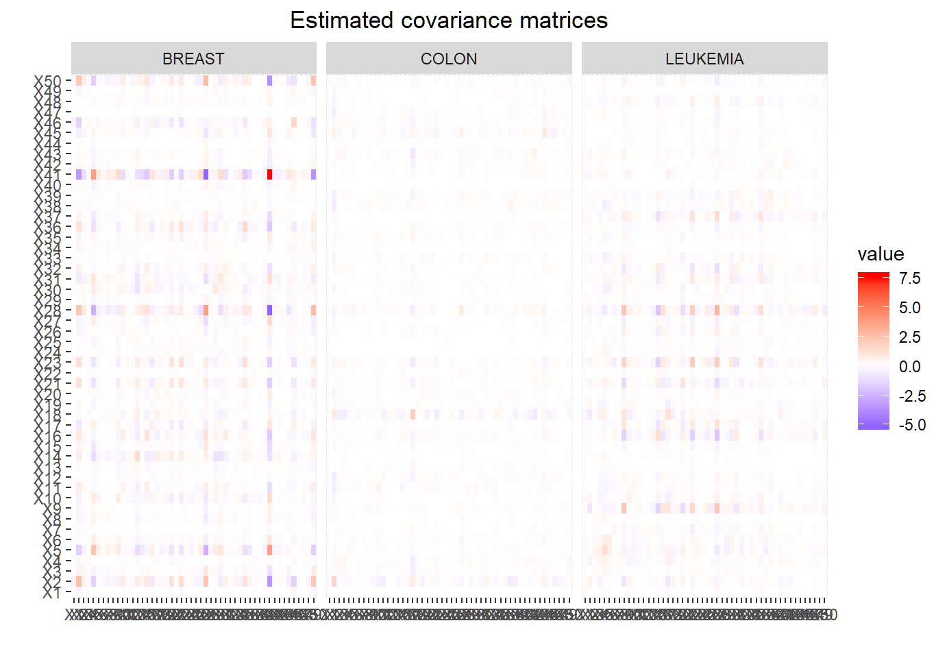
Plot est. covariance matrices

> library(ggplot2)
> ggplot(data=EstSigmaAll, aes(x=Var1, y=Var2, fill=value)) + 
+   geom_tile()+scale_fill_gradient2(low="blue", high="red")+
+   facet_grid(~Cancer)+xlab("")+ylab("")+
+   ggtitle("Estimated covariance matrices")+
+   theme(plot.title = element_text(hjust = 0.5))

ggplot(...,aes(x=, y=, fill=value)) should be used with xlab("")+ylab("") since no x-axis or y-axis label is needed
feature variables will be shown on both axes since pairwise covariances are computed for them
resulting plot is similar to a heatmap

Visualization of est. cov. matrx.

Much less dependence among genes for “COLON” cancer than for “BREAST” or “LEUKEMIA” cancer

Discriminant analysis: Example 4

Stock market data

Data set Smarket{ISLR} contains observations for S&P 500 stock index over 1,250 days, from the beginning of 2001 until the end of 2005, such as

percentage returns for each of the five previous trading days, as Lag1 through Lag5
Direction (whether market was Up or Down on this date)

> library(ISLR); dim(Smarket)
[1] 1250    9
> Smarket[1,]
  Year  Lag1   Lag2   Lag3   Lag4 Lag5 Volume Today Direction
1 2001 0.381 -0.192 -2.624 -1.055 5.01 1.1913 0.959        Up
> levels(Smarket$Direction)
[1] "Down" "Up"

Target: predict market Direction using Lag1 and Lag2

LDA: training

Model: 2 features $X_1=$Lag1 and $X_2=$Lag2; 2 component bivariate Gaussian densities $f_1 \sim \text{Gaussian}(\mu_1,\Sigma_1)$ and $f_2 \sim \text{Gaussian}(\mu_2,\Sigma_2)$; 2 mixing proportions (as priors) $\pi_1$ and $\pi_2$; 2 classes Down and Up

> train=(Smarket$Year<2005); Smarket.2005=Smarket[!train,]
> Direction.2005=Smarket$Direction[!train]
> library(MASS)
> lda.fit=lda(Direction~Lag1+Lag2,data=Smarket,subset=train)

observations from 2001 through 2004 as training set
note the use of subset=train in lda
LDA assumes $\Sigma_1=\Sigma_2$

LDA: estimated model

Estimated prior (i.e., mixing) probabilities and mean vectors:

Prior probabilities of groups:
    Down       Up 
0.491984 0.508016 

Group means:
            Lag1        Lag2
Down  0.04279022  0.03389409
Up   -0.03954635 -0.03132544

Class 1 is Direction=Down; Class 2 is Direction=Up
$\hat{\pi}_1=0.492$, $\hat{\pi}_2=0.508$, $\hat{\mu}_1=(0.0428,0.0339)^T$, $\hat{\mu}_2=(-0.0395,-0.0313)^T$

LDA: estimated model

Recall the estimated linear discriminant function as \[\hat{\delta}_{k}(x)=x^T \underbrace{\hat{\Sigma}^{-1}\hat{\mu}_k}_{\hat{c}_k} -\frac{1}{2} \hat{\mu}_k^T \underbrace{\Sigma^{-1}\hat{\mu}_k}_{\hat{c}_k} + \log \hat{\pi}_k, k \in \mathcal{G}\]

Coefficients of linear discriminants:
            LD1
Lag1 -0.6420190
Lag2 -0.5135293

$\hat{c}_2=(-0.642,-0.514)^T$, since Class 2 is Direction=Up and Up $\mapsto 1$ (and Class 1 as Direction=Down and Down$\mapsto 0$)

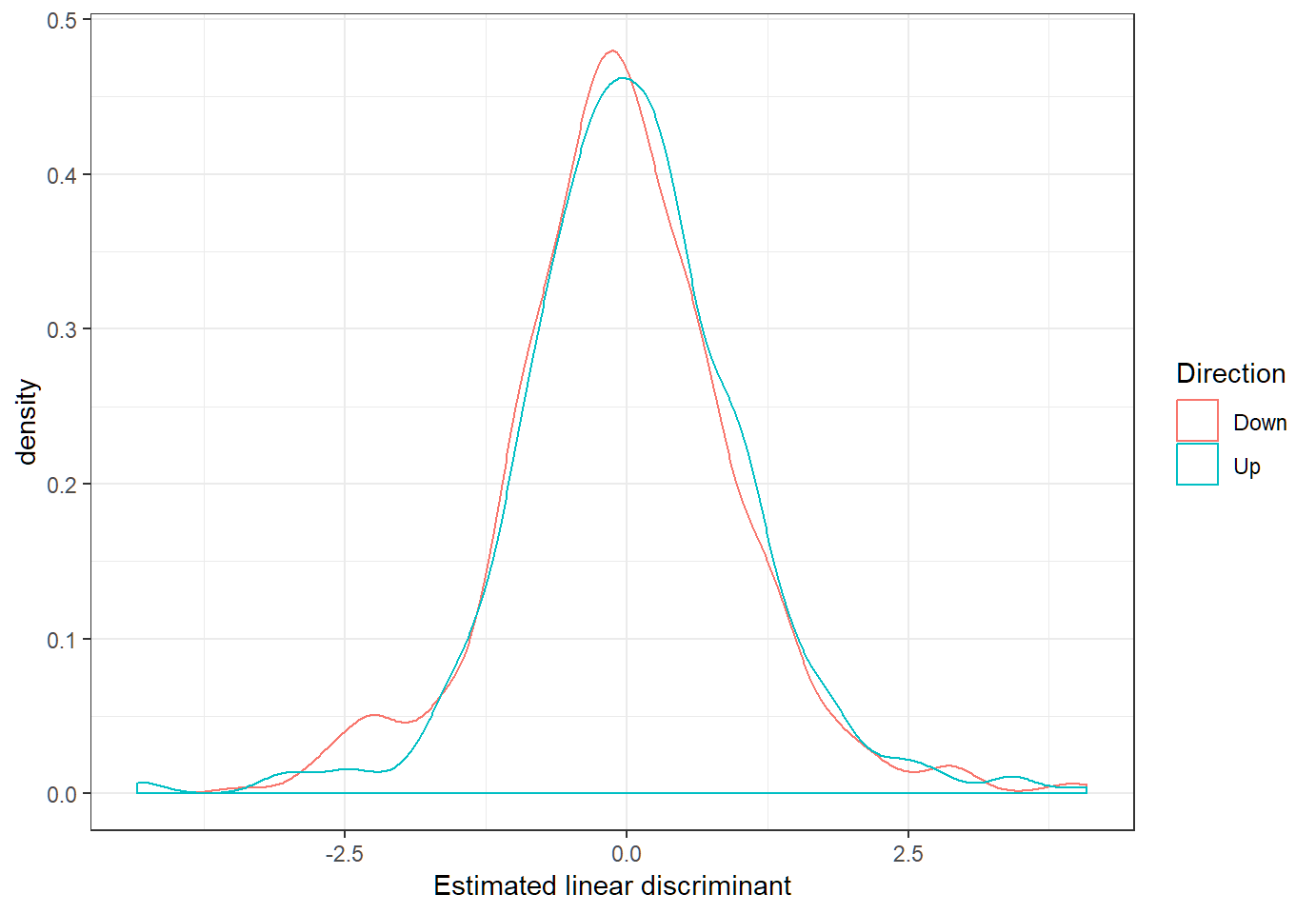
Linear discriminants

Define estimated linear discriminant as $\hat{d}_{k}(x)=x^T \hat{c}_k,k \in \mathcal{G}$

LDA: predicting

Classification on test set Smarket.2005:

> dim(Smarket.2005)
[1] 252   9
> lda.pred=predict(lda.fit, Smarket.2005)
> names(lda.pred)
[1] "class"     "posterior" "x"        
> lda.class=lda.pred$class
> table(lda.class,Direction.2005)
         Direction.2005
lda.class Down  Up
     Down   35  35
     Up     76 106
> mean(lda.class==Direction.2005)
[1] 0.5595238

lda.pred$x: vector of estimated linear discriminant for each observation
classwise error rates: Down and Up respectively

[1] 0.6846847 0.2482270

QDA: estimated model

> qda.fit=qda(Direction~Lag1+Lag2,data=Smarket,subset=train)
> qda.fit
Call:
qda(Direction ~ Lag1 + Lag2, data = Smarket, subset = train)

Prior probabilities of groups:
    Down       Up 
0.491984 0.508016 

Group means:
            Lag1        Lag2
Down  0.04279022  0.03389409
Up   -0.03954635 -0.03132544

qda does not produce “coefficients of linear discriminants” since it uses a quadratic decision boundary
estimated prior (i.e., mixing) probabilities and mean vectors are the same as those obtained by LDA

QDA: predicting

Classification on test set Smarket.2005:

> qda.class=predict(qda.fit,Smarket.2005)$class
> table(qda.class,Direction.2005)
         Direction.2005
qda.class Down  Up
     Down   30  20
     Up     81 121
> mean(qda.class==Direction.2005)
[1] 0.5992063

around 60% (average) accuracy of QDA, in comparison with around 56% (average) accuracy of LDA
QDA: impressive performance for these stock market data

License and session Information

License

> sessionInfo()
R version 3.5.0 (2018-04-23)
Platform: x86_64-w64-mingw32/x64 (64-bit)
Running under: Windows 10 x64 (build 19041)

Matrix products: default

locale:
[1] LC_COLLATE=English_United States.1252 
[2] LC_CTYPE=English_United States.1252   
[3] LC_MONETARY=English_United States.1252
[4] LC_NUMERIC=C                          
[5] LC_TIME=English_United States.1252    

attached base packages:
[1] stats     graphics  grDevices utils     datasets  methods  
[7] base     

other attached packages:
[1] knitr_1.21

loaded via a namespace (and not attached):
 [1] compiler_3.5.0  magrittr_1.5    tools_3.5.0    
 [4] htmltools_0.3.6 revealjs_0.9    yaml_2.2.0     
 [7] Rcpp_1.0.0      stringi_1.2.4   rmarkdown_1.11 
[10] highr_0.7       stringr_1.3.1   xfun_0.4       
[13] digest_0.6.18   evaluate_0.12

Stat 437 Lecture Notes 5c

Xiongzhi Chen

Washington State University

Discriminant analysis: Example 3

Human cancer microarray data

Obtain subset of data

Glimpse on subset of data

Visualize subset of data

Visualize subset of data

LDA: p > 2n

QDA: p > 2n

Singular DA: p > n

Regularized DA

Regularized DA via klaR

Regularized DA via klaR

Regularized DA via klaR

Regularized DA via klaR

Extract est. covariance matrices

Melt est. covariance matrices

Plot est. covariance matrices

Visualization of est. cov. matrx.

Discriminant analysis: Example 4

Stock market data

LDA: training

LDA: estimated model

LDA: estimated model

Linear discriminants

LDA: predicting

QDA: estimated model

QDA: predicting

License and session Information

Regularized DA via `klaR`

Regularized DA via `klaR`

Regularized DA via `klaR`

Regularized DA via `klaR`