Overview

Support vector machine is a generalization of the classifier that uses a hyperplane to perfectly separate observations into classes.

The contents on support vector machine are adapted or adopted from:

• mainly Chapter 9 of the Text “An Introduction to Statistical Learning with Applications in R (Corrected at 8th printing)”
• partially Chapter 12 of the Supplementary Text “The Elements of Statistical Learning: Data Mining, Inference, and Prediction (2nd Edition)”
• other sources

Learning submoduels

Subtopics to be covered:

• Hyperplane and related geometry
• Maximal margin classifier
• Support vector classifier
• Support vector machine (SVM)
• Software implementation of SVM

Hyperplane

A hyperplane \(S\)

• in \(\mathbb{R}^1\) is a single point
• in \(\mathbb{R}^2\) is a line, defined by \[S=\left\{x=(x_1,x_2)^T \in \mathbb{R}^2: a x_1+bx_2+d=0\right\}\] with \(\vert a\vert+\vert b\vert >0\)
• in \(\mathbb{R}^3\) is a plane, defined by \[S=\left\{x=(x_1,x_2,x_3)^T \in \mathbb{R}^3: a x_1+b x_2+c x_3+d=0\right\}\] with \(\vert a\vert+\vert b \vert +\vert c \vert>0\)

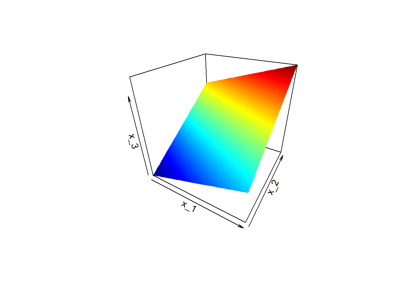
Hyerplane in 3D

Plane \(S = \{x=(x_1,x_2,x_3)^T \in \mathbb{R}^3: x_3 = x_1 + 2 x_2 -1\}\)

Hyperplane and inner product

• In the \(p\)-dimensional Euclidean space \(\mathbb{R}^p\), a hyperplane \(S\) is an affine, linear subspace of dimension \(p-1\), where “affine” indicates that \(S\) need not pass through the origin.

• Let \(x=(x_1,x_2,\ldots,x_p)^T\) for \(x \in \mathbb{R}^p\). The definition is \[S=\left\{x \in \mathbb{R}^p: \beta_1 x_1+\beta_2 x_2+\ldots+\beta_px_p+\beta_0=0 \right\},\] where \(\sum_{j=1}^p\vert \beta_j\vert>0\); otherwise, \(S\) will have dimension less than \(p-1\)

• Write \(\alpha=(\beta_1,\ldots,\beta_p)^T\). Recall the inner product \(\langle x,\alpha\rangle=x^T \alpha\) and norm \(\Vert \alpha\Vert = \sqrt{\sum_{j=1}^p \beta_j^2}\) in \(\mathbb{R}^p\) . Then \[S=\left\{x \in \mathbb{R}^p: \langle x,\alpha\rangle = - \beta_0, \Vert \alpha\Vert >0 \right\}\]

Hyperplane and orientation

In the \(p\)-dimensional Euclidean space \(\mathbb{R}^p\), a hyperplane \(S\) is determined by a vector \(\alpha \in \mathbb{R}^p\) with \(\Vert \alpha\Vert >0\) and a scalar \(\beta_0\) such that \(S\) contains vectors \(x \in \mathbb{R}^p\) whose inner products with \(\alpha\) are \(-\beta_0\). Namely, \[S=\left\{x \in \mathbb{R}^p: \langle x,\alpha\rangle = - \beta_0 \right\}.\] Let us call \(\alpha\) the “direction” and \(\beta_0\) the “intercept” of \(S\)

Because the inner product of two vectors is related to the angle between them, we see \(S\) splits \(\mathbb{R}^p\) into halves as

• One side \(S_{+} = \left\{ x \in \mathbb{R}^p: \langle x,\alpha\rangle > - \beta_0 \right\}\)
• Other side \(S_{-} = \left\{ x \in \mathbb{R}^p: \langle x,\alpha\rangle < - \beta_0 \right\}\)

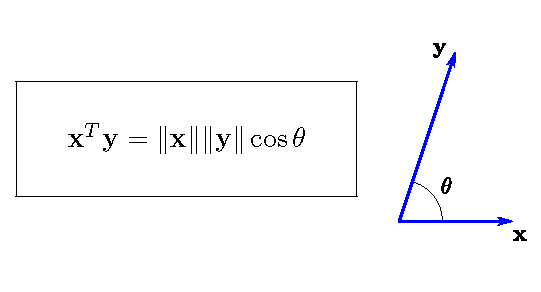
Inner product and angle

For \(\mathbf{x},\mathbf{y} \in \mathbb{R}^p\), \(\langle \mathbf{x},\mathbf{y}\rangle = \mathbf{x}^T \mathbf{y}\). So, \(\langle \mathbf{x},\mathbf{y}\rangle >0\) if \(-\pi/2<\theta < \pi/2\), and \(\langle \mathbf{x},\mathbf{y}\rangle=\cos\theta\) if \(\Vert \mathbf{x}\Vert=\Vert \mathbf{y} \Vert =1\).

Inner product and angle

• The identity \(\langle x,\alpha\rangle = - \beta_0\) for a hyperplane \(S\) in \(\mathbb{R}^p\) is equivalent to

\[ \left \langle \frac{x}{\Vert x \Vert},\frac{\alpha}{\Vert \alpha \Vert} \right \rangle = \left \langle \tilde{x}, \tilde{\alpha} \right \rangle = \frac{- \beta_0}{\Vert x \Vert \Vert \alpha \Vert} = c \] where both \(\tilde{x} = {x}/{\Vert x \Vert}\) and \(\tilde{\alpha} ={\alpha}/{\Vert \alpha \Vert}\) have norm \(1\) and have the same directions as \(x\) and \(\alpha\), respectively

• So, which side of \(S\) \(\tilde{x}\) (and hence \(x\)) is on depends on the sign of \(\left \langle \tilde{x}, \tilde{\alpha} \right \rangle-c\) (i.e., the sign of \(\langle x,\alpha\rangle + \beta_0\))

Note: the sign of a number \(a \in \mathbb{R}\) is denoted by \(\operatorname*{sgn}{a}\), and \(\operatorname*{sgn}{a}=1\) if \(a>0\), \(=0\) if \(a=0\), and \(=-1\) if \(a<0\)

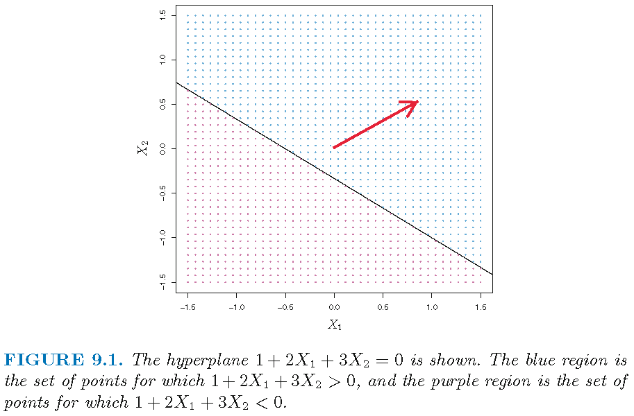
Hyperplane and splits

Hyperplane \(S\) via \(\alpha = (\beta_1,\beta_2)^T =(2,3)^T\) and \(\beta_0 =1\); red vector is \(\tilde{\alpha} ={\alpha}/{\Vert \alpha \Vert}=(0.555,0.832)^T\):

Classification task

Training set \(\mathcal{T}\) of \(n\) observations \((x_{1},y_{1}),\ldots,(x_{n},y_{n})\)

• \(x_{i}\in \mathbb{R}^{p}\) records the \(i\)th observation for the same \(p\) features
• \(y_{i}\in \mathcal{G}=\{-1,1\}\) is the class label for \(x_{i}\), and \(1,-1\) are the class labels

The task: for a test observation \((x_0,y_0)\) with known \(x_0\in\mathbb{R}^{p}\) but unknown \(y_0\in \mathcal{G}\), classify \(x_0\) into one of the \(2\) classes by estimating \(y_0\)

Note: labels \(-1\) and \(1\) are set with respect to the orientation determined by a hyperplane

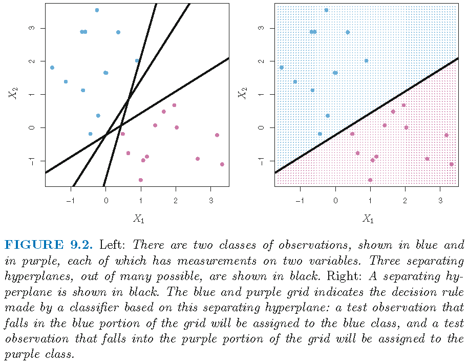
Separating hyperplane

• Recall \(\alpha=(\beta_1,\ldots,\beta_p)^T\), the hyperplane \[S =\left\{x \in \mathbb{R}^p: \langle x,\alpha\rangle + \beta_0 =0\right\}\] and its “two sides” \[ \begin{aligned} S_{+} =\left\{x \in \mathbb{R}^p: \langle x,\alpha\rangle + \beta_0 >0 \right\}\\ S_{-} =\left\{x \in \mathbb{R}^p: \langle x,\alpha\rangle + \beta_0 <0 \right\} \end{aligned} \]
• \(S\) is called a separating hyperplane for observations \(\{(x_{i},y_{i})\}_{i=1}^n\) if \(y_i=1\) for \(x_i \in S_{+}\) and \(y_i=-1\) for \(x_i \in S_{-}\), i.e., if \[ y_i (\langle x_i,\alpha\rangle + \beta_0) >0 , \forall i \]

Note: \(\operatorname*{sgn}{(y_i)} = \operatorname*{sgn}{(\langle x_i,\alpha\rangle + \beta_0)}\) for a separating hyperplane \(S\)

Separating hyperplane

“Hyperplane” classifier

• Let \(x_0 = (x_{01},\ldots,x_{0p})^T\). If a separating hyperplane \(S\) exists, the we can assign \(x_0\) to a class depending on which side of the hyperplane it is located, i.e., by setting \[ \hat{y}_0 = \operatorname*{sgn}(\langle x_0,\alpha\rangle + \beta_0). \] This gives a “hyperplane” classifier

• For a set of observations that can be perfectly separately by a hyperplane, there can be infinitely many separating hyperplanes and hence infinitely many “hyperplane” classifiers for these observations

• Each “hyperplane” classifier has a twin that is obtained by flipping the two sides of the hyperplane

“Hyperplane” classifier

Maximal margin classifier

• If training observations can be perfectly separately by a hyperplane, then there are infinitely many separating hyperplanes and hence infinitely many “hyperplane” classifiers for these observations
• So, we choose the optimal hyperplane that is the farthest from the training observations. Here the distance of a set of observations to a hyperplane is the minimum of the distance of an observation in the set to the hyperplane, and the distance of the training set to a hyperplane is also called the margin
• This optimal hyperplane is called maximal margin hyperplane and its induced classifier called maximal margin classifier

Maximal margin classifier

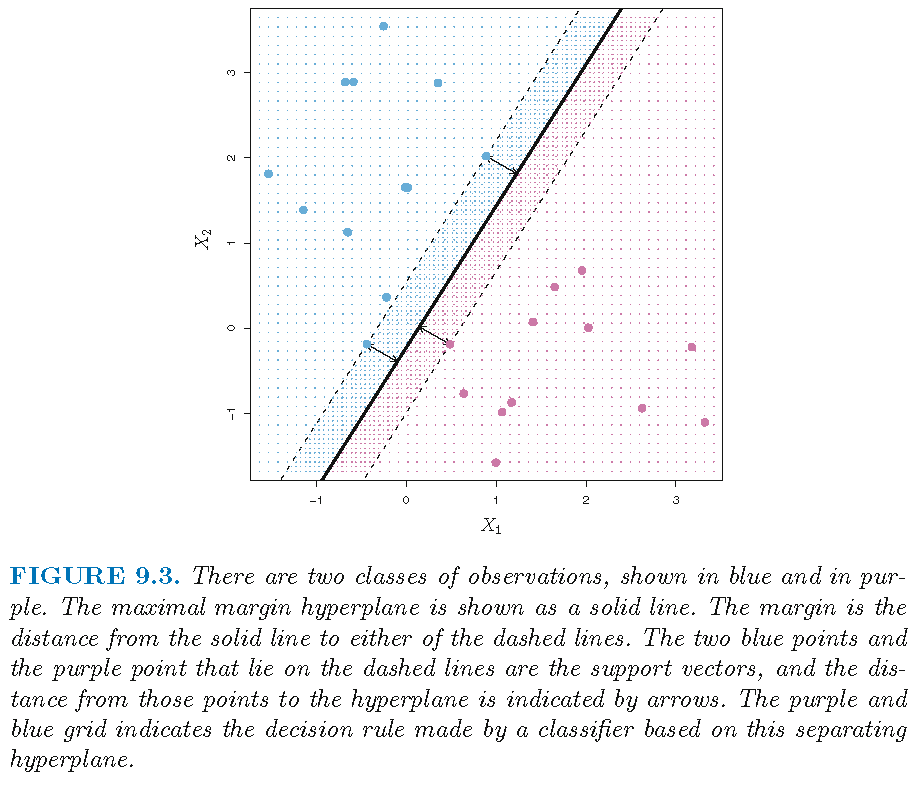
Support vectors

Support vectors are training observations that achieve the maximal margin with respect to the optimal hyperplane

Support vectors

Support vectors

• are training observations that achieve the maximal margin with respect to the optimal hyperplane
• “support” the maximal margin hyperplane in the sense that if these points were moved slightly then this hyperplane would move as well
• determine the maximal margin hyperplane in the sense that a movement of any of the other observations not cross the boundary set by the margin would not affect the separating hyperplane

Maximal margin classifier

• Recall training set \(\mathcal{T}=\left\{ (x_{1},y_{1}),\ldots,(x_{n},y_{n}) \right\}\)
• Let \(\operatorname*{dist}\) be the distance function. The distance from \(\mathcal{T}\) to a separating hyperplane \(S\) is (by definition) \[ \operatorname*{dist}(\mathcal{T},S)=\min\nolimits_{x_i \in \mathcal{T}} \operatorname*{dist}(x_i,S) \]
• The maximal margin hyperplane is \[ \begin{aligned} \hat{S} & = \operatorname*{argmax}\nolimits_{S \in \mathcal{S}} \operatorname*{dist}(\mathcal{T},S)\\ & = \{x \in \mathbb{R}^p: \langle x,\hat{\alpha}\rangle + \hat{\beta}_0=0\} \end{aligned} \] with direction \(\hat{\alpha}\) and intercept \(\hat{\beta}_0\)
• The maximal margin classifier assigns \(x_0\) to class \(\hat{y}_0\) with \[ \hat{y}_0 = \operatorname*{sgn}(\langle x_0,\hat{\alpha}\rangle + \hat{\beta}_0) \]

Intuition on optimal hyperplane

Under separability hypothesis that observations in \(\mathcal{T}=\left\{ (x_{1},y_{1}),\ldots,(x_{n},y_{n}) \right\}\) can be perfectly separated by a hyperplane \(S\):

• let \(T_1=\{x_i:y_i=1\}\) and \(T_{-1}=\{x_i:y_i=-1\}\)
• since \[ \begin{aligned} \operatorname*{dist}(T_{1},S)=\min\nolimits_{x_i \in T_{1}}\operatorname*{dist}(x_i,S)=\operatorname*{dist}(\hat{x},S)\\ \operatorname*{dist}(T_{-1},S)=\min\nolimits_{x_i \in T_{-1}}\operatorname*{dist}(x_i,S)= \operatorname*{dist}(\tilde{x},S) \end{aligned} \] for some \(\hat{x} \in T_{1}\) and \(\tilde{x} \in T_{-1}\), then (to be continued)

Remark: in the expression for \(\operatorname*{dist}(T_{1},S)\), the 1st equality is the definition, and the 2nd due to the finite sample size of \(\mathcal{T}\). Similar reasoning holds for \(\operatorname*{dist}(T_{-1},S)\)

Intuition on optimal hyperplane

then \[ \begin{aligned} \operatorname*{dist}(\mathcal{T},S) & = \min\nolimits_{x_i \in \mathcal{T}}\operatorname*{dist}(x_i,S)\\ & =\min \{\operatorname*{dist}(T_{1},S),\operatorname*{dist}(T_{-1},S)\}\\ & = \min \{\operatorname*{dist}(\hat{x},S),\operatorname*{dist}(\tilde{x},S)\} \end{aligned} \]

Remark: in the expression for \(\operatorname*{dist}(\mathcal{T},S)\), the 1st equality is the definition, the 2nd due to the hypothesis that observations in \(\mathcal{T}\) can be perfectly separated by a hyperplane \(S\), and the 3rd due to the previous bullet point

• In summary, for some \(\hat{x} \in T_{1}\) and \(\tilde{x} \in T_{-1}\), \[ \begin{aligned} \operatorname*{dist}(\mathcal{T},S) = \min \{\operatorname*{dist}(\hat{x},S),\operatorname*{dist}(\tilde{x},S)\} \end{aligned} \] for a separating hyperplane \(S\)

Intuition on optimal hyperplane

Under the “separability hypothesis”, we have \[\operatorname*{dist}(\mathcal{T},S) = \min \{\operatorname*{dist}(\hat{x},S),\operatorname*{dist}(\tilde{x},S)\}\] for some \(\hat{x} \in T_{1}\) and \(\tilde{x} \in T_{-1}\). So, \(\hat{S}\) has to lie in the “gap” between \(\hat{x}\) and \(\tilde{x}\) and evenly split the gap:

• because if \(\hat{S}\) does not evenly split the gap, then one among \(\operatorname*{dist}(T_{1},\hat{S})\) and \(\operatorname*{dist}(T_{-1},\hat{S})\) is bigger than the other, e.g., \(\operatorname*{dist}(T_{1},\hat{S}) > \operatorname*{dist}(T_{-1},\hat{S})\), and in this case we must have \[\operatorname*{dist}(\mathcal{T},\hat{S})=\operatorname*{dist}(T_{-1},\hat{S}).\] Now if we parallelly move \(\hat{S}\) towards \(T_1\), then \(\operatorname*{dist}(T_{-1},\hat{S})\) (and hence \(\operatorname*{dist}(\mathcal{T},\hat{S})\)) is strictly increased, contracting \(\operatorname*{dist}(\mathcal{T},\hat{S})\) being the largest

Intuition on support vectors

For maximal margin hyperplane \(\hat{S}\),

• the observations \(\hat{x} \in T_{1}\) and \(\tilde{x} \in T_{-1}\) such that \[ \begin{aligned} & \operatorname*{dist}(T_{1},\hat{S})=\operatorname*{dist}(\hat{x},\hat{S}) \\ = & \ \operatorname*{dist}(T_{-1},\hat{S})= \operatorname*{dist}(\tilde{x},\hat{S})=0.5 \times \operatorname*{dist}(\mathcal{T},\hat{S}) \end{aligned} \] are exactly the support vectors

• the two hyperplanes that are parallel to \(\hat{S}\), that are on the opposite sides of \(\hat{S}\), and that pass through the support vectors form the margin or boundary (for classification)

Intuition on optimal hyperplane

Construction via optimization

Under “separability hypothesis” on the training set \(\mathcal{T}=\{(x_{1},y_{1}),\ldots,(x_{n},y_{n})\}\), the maximal margin classifier \(\hat{S}\) with direction \(\hat{\alpha}\) and intercept \(\hat{\beta_0}\) is the solution of the following optimization problem:

\[ \begin{aligned} &\quad \quad \quad \max_{\beta_{0} \in \mathbb{R},\alpha \in \mathbb{R}^p,M}M\\ \text{subject to: } & \text{(C1.)} \quad \Vert \alpha \Vert=1,\\ &\text{(C2.)} \quad \min_{1\leq i\leq n}y_{i}\left( \langle x_{i}, \alpha \rangle+\beta_{0}\right) \geq M \end{aligned} \]

Note: if \(\alpha \in \mathbb{R}^p\) and \(\Vert \alpha \Vert=1\), we also write \(\alpha \in S^{p-1}\), the sphere of radius \(1\) in \(\mathbb{R}^p\)

Explanation on constraints

Write the hyperplane \(S\) with direction \(\alpha\) and intercept \(\beta_0\) as \(S(\alpha,\beta_0)\). Then

• when \(M>0\), the constraint \[ \min_{1\leq i\leq n}y_{i}\left(\langle x_{i}, \alpha \rangle+\beta_{0}\right) \geq M \] ensures that each observation will be on the correct side of \(S(\alpha,\beta_0)\)
• the constraint \(\Vert \alpha \Vert=1\) ensures that the distance of \(x_i\) to \(S(\alpha,\beta_0)\) is exactly \(y_{i}\left(\langle x_{i}, \alpha \rangle+\beta_{0}\right)\), i.e., \[\text{dist}(x_i,S(\alpha,\beta_0))=y_{i}\left(\langle x_{i}, \alpha \rangle+\beta_{0}\right)\]

Normal vector of hyperplane

The normal vector \(\mathbf{n}\) (“normal” for short) to a hyperplane is a vector which is perpendicular (via inner product) to the hyperplane, i.e., \(\langle \mathbf{n}, \mathbf{r-r_0}\rangle = 0\) (Credit: normal vector)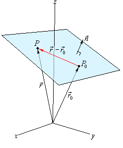

Normal vector and distance

\(\text{dist}(P,S)\) is the orthogonal projection of \(\overrightarrow{QP}\) with \(Q \in S\) onto the normal \(\mathbf{n}\) and is equal to \(\Vert\overrightarrow{RP}\Vert\) (Credit: planes)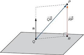

Normal vector and distance

• For a hyperplane \(S =\left\{x \in \mathbb{R}^p: \langle x,\alpha\rangle + \beta_0 =0\right\}\), its normal is \(\alpha\) (which is why we call \(\alpha\) the “direction”)

• For any point \(x_0 \in \mathbb{R}^p\), its distance to \(S\) is \[\text{dist}(x_0,S)= \vert \langle x_0, \alpha\rangle + \beta_0 \vert/\Vert \alpha \Vert \]

• Since the class label \(y_0 \in \{-1,1\}\) for \(x_0\) satisfies \[\operatorname*{sgn}(y_0) = \operatorname*{sgn}(\langle x_0, \alpha \rangle + \beta_0),\] when \(\Vert \alpha \Vert=1\), we have \[ \text{dist}(x,S)=y_0 (\langle x_0, \alpha \rangle+\beta_0), \] as claimed by the Text (on page 343)

Credit: normal vector and distance to plane

Summary of construction

The maximal margin classifier \(\hat{S}(\hat{\alpha},\hat{\beta}_0)\) solves the optimization problem:

\[ \begin{aligned} &\quad \max_{\beta_{0} \in \mathbb{R},\alpha \in S^{p-1},M \in \mathbb{R}^{+}}M\\ \text{subject to: } & \underbrace{\min_{1\leq i\leq n} \underbrace{y_{i}\left(\langle x_{i}, \alpha \rangle+\beta_{0}\right)}_{\text{distance of } x_i \text{ to } S(\alpha,\beta_0)}}_{\text{distance of training set } \mathcal{T} \text{ to } S(\alpha,\beta_0)} \geq M \end{aligned} \]

where \(S^{p-1} = \{x \in \mathbb{R}^p: \Vert x \Vert=1\}\), \(\mathbb{R}^{+}=\{t\in \mathbb{R}: t>0\}\) and \(S(\alpha,\beta_0)\) is the hyperplane with direction \(\alpha\) and intercept \(\beta_0\)

Non-separability

Maximal margin classifier undefined when observations cannot be perfectly separately by a hyperplane:

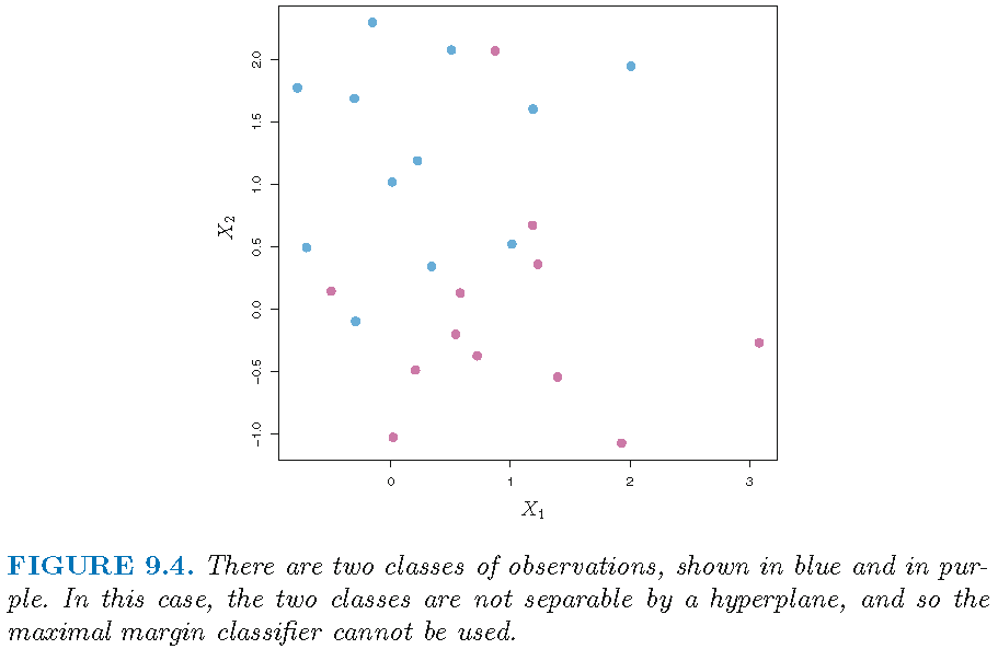
Support vector classifiers

• When observations cannot be perfectly separately by a hyperplane (which is called the “non-separable case”), the optimization problem for the maximal margin classifier has no solution, and the maximal margin classifier is undefined

• So, we aim to develop a hyperplane that almost separates the classes, using a so-called soft margin. The generalization of the maximal margin classifier to the non-separable case is known as the support vector classifier

Recap: maximal margin classifier

Every observation is on the correct side of the maximal margin hyperplane and on the correct side of the margin

Recap: maximal margin classifier

The maximal margin classifier achieves perfect and maximal margin separation, i.e., every observation is not only on the correct side of the maximal margin hyperplane but also on the correct side of the margin.

However, due to maximal margin separation,

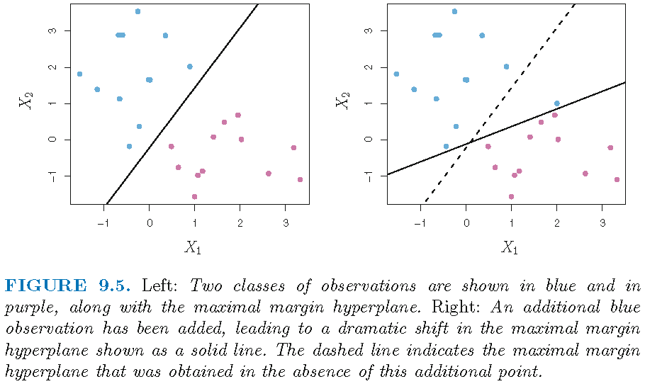
• the classifier is very sensitive to a change in a support vector or single observation that is close to the boundary (set by the maximal margin), and may overfit the training data

• the classifier is undefined in the non-separable case where observations cannot be perfectly separately by a hyperplane

Recap: maximal margin classifier

Sensitivity to observations on boundary or close to margin:

Support vector classifiers

To alleviate some issues of the maximal margin classifier, the support vector classifier, sometimes called a soft margin classifier,

• uses a hyperplane that does not perfectly separate the two classes, and is applicable when there is no separating hyperplane for the two classes

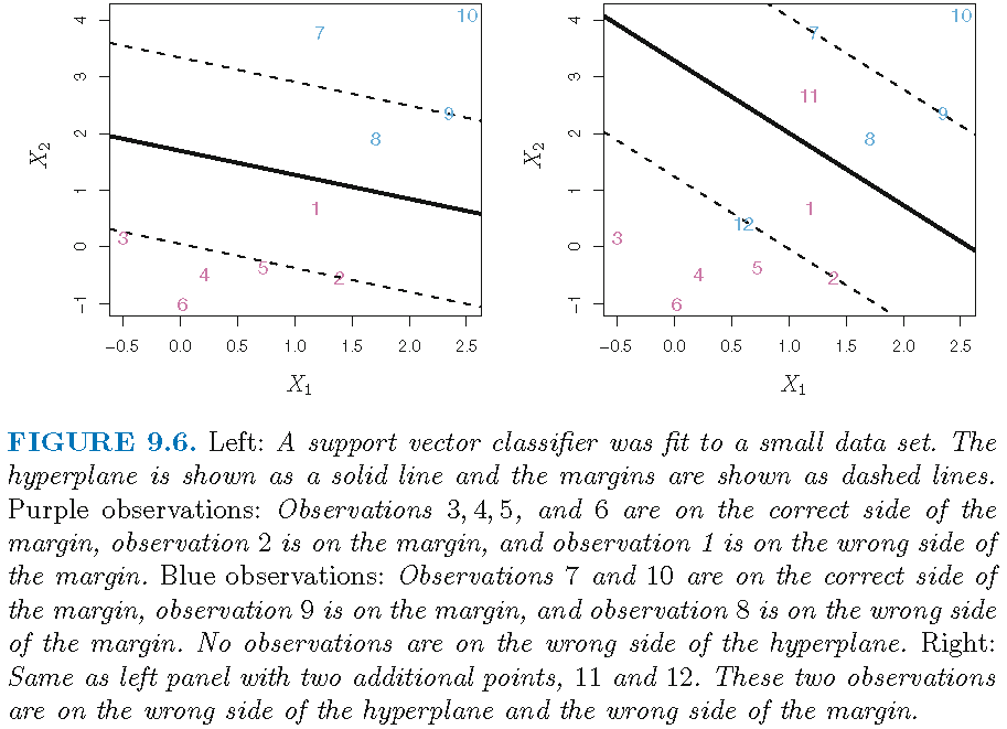
• allows some observations to be on the incorrect side of the margin, or even the incorrect side of the hyperplane, and achieves greater robustness to individual observations. (The margin is soft because it can be violated by some of the training observations)

Support vector classifiers

Soft margin and imperfect separation:

Construction

• The optimal hyperplane \(\hat{S}=\hat{S}(\hat{\alpha},\hat{\beta}_0)\) with direction \(\hat{\alpha}\) and intercept \(\hat{\beta}_0\) solves the optimization problem: \[ \begin{aligned} &\quad \max_{\beta_{0} \in \mathbb{R},\alpha \in S^{p-1},M \in \mathbb{R}^{+}}M\\ \text{subject to: } & \forall i, \underbrace{y_{i}\left( \langle x_{i}, \alpha \rangle +\beta_{0}\right)}_{\text{distance from } x_i \text{ to } S(\alpha,\beta_0)} \geq \underbrace{M\left( 1-\epsilon_{i}\right)}_{\text{proportional margin}}\\ & \underbrace{\epsilon_{i}\geq 0,\forall i; \sum\nolimits_{i=1}^n\epsilon_{i}\leq C}_{\text{amount of violation}} \text{ for some } C>0 \\ \end{aligned} \]
• The support vector classifier assigns \(x_0\) to class \[ \hat{y}_0 = \operatorname*{sgn}(\langle x_0,\hat{\alpha}\rangle + \hat{\beta}_0) \]

Slack variables

• \(M\) is the margin, as in the optimization to obtain the maximal margin classifier

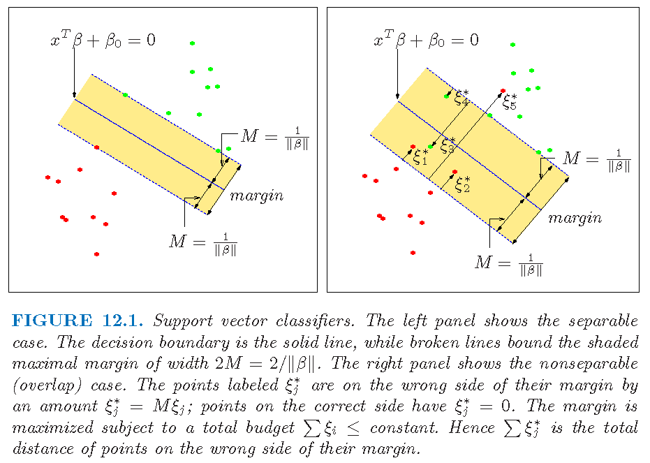
• The \(\epsilon_{i}\)’s are slack variables that allow individual observations to be on the wrong side of the margin or the hyperplane. Specifically, \[ \epsilon_{i} = \left\{ \begin{array} {lll} 0 & \implies & x_i \text{ is on correct side of margin} \\ \in (0,1] & \implies & x_i \text{ is on wrong side of margin} \\ & & \text{but on correct side of hyperplane} \\ > 1 & \implies & x_i \text{ is on wrong side hyperplane} \end{array}\right. \]

Slack variables

Figure 12.1 of Supplementary Text (\(\beta=\alpha,\xi_i=\epsilon_i\)):

Tolerance of violation

• The \(C>0\) in \(\sum_{i=1}^n\epsilon_{i}\leq C\) controls the number and severity of violations to the margin and to the hyperplane by the predicted class labels. \(C\) is a constant and referred to as the “tolerance” or budget. \[ C = \left\{ \begin{array} {lll} 0 & \implies & \text{all }\epsilon_i = 0 \text{ and optimization is}\\ & & \text{as for maximal margin classifier} \\ >0 & \implies & \text{ no more than } C \ x_i's \\ & & \text{ are on wrong side of hyperplane} \\ \uparrow & \implies & \text{ more tolerant of violations; wider margin} \end{array}\right. \]

• \(C\) is a tuning parameter and is often chosen via cross-validation

Support vectors

Summary on optimization and optimal hyperplane:

• Observations that lie directly on the margin or on the wrong side of the margin for their class, known as support vectors, affect the optimal hyperplane and hence the induced support vector classifier

• An observation that lies far away from the optimal hyperplane (and far away from the margin) does not affect much the hyperplane or hence the induced support vector classifier, and changing the position of that observation would not change the classifier at all, provided that its position remains on the correct side of the margin

Support vectors and tolerance

Since the support vector classifier is only affected by support vectors, the tuning parameter \(C\) controls the bias-variance trade-off of the classifier as follows:

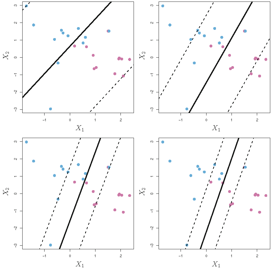
• When \(C\) is large, then the margin is wide, many observations can violate the margin, and so there are many support vectors jointly determining the hyperplane. In this case, the classifier is more stable to changes to individual observations (i.e., smaller variance) but has larger classification error (i.e., larger bias)
• In contrast, if \(C\) is small, then there will be fewer support vectors and hence the resulting classifier will have low bias but high variance

Margin and tolerance

Figure 9.7 of Text: support vector classifier with varying tolerance \(C\); larger \(C\), wider margin

An equivalence

• Consider \(\quad \max_{\beta_{0} \in \mathbb{R},\alpha \in S^{p-1},M \in \mathbb{R}^{+}}M \quad\) subject to \[ \begin{aligned} \min_{1\leq i\leq n}y_{i}\left( \langle x_{i}, \alpha \rangle+\beta_{0}\right) \geq M \end{aligned} \]
• Transforming \[ \alpha \mapsto \alpha^{\prime}=\alpha/M, \quad \beta_{0}\mapsto\beta_{0}^{\prime}=\beta_{0}/M \] gives \(\Vert \alpha^{\prime} \Vert=M^{-1}\) and \[ \max_{\beta_{0} \in \mathbb{R},\alpha \in S^{p-1},M \in \mathbb{R}^{+}}M = \min_{\beta_{0}^{\prime} \in \mathbb{R},\alpha^{\prime} \in \mathbb{R}^{p}}\left\Vert \alpha^{\prime}\right\Vert \] subject to \[ \begin{aligned} \min_{1\leq i\leq n}y_{i}\left( \langle x_{i}, \alpha^{\prime} \rangle+\beta_{0}^{\prime}\right) \geq 1 \end{aligned} \]
• However, \[\operatorname*{argmin}\nolimits_{\beta_{0}^{\prime} \in \mathbb{R},\alpha^{\prime} \in \mathbb{R}^{p}}\left\Vert \alpha^{\prime}\right\Vert = \operatorname*{argmin}\nolimits_{\beta_{0}^{\prime} \in \mathbb{R},\alpha^{\prime} \in \mathbb{R}^{p}} 2^{-1}\left\Vert \alpha^{\prime}\right\Vert^2\]

The equivalence for MMC

The equivalence between two optimization problems to obtain maximal margin classifier (MMC):

• Optimization: \(\quad \max_{\beta_{0} \in \mathbb{R},\alpha \in S^{p-1},M \in \mathbb{R}^{+}}M\) \[ \begin{aligned} \text{subject to}\quad \min_{1\leq i\leq n}y_{i}\left( \langle x_{i}, \alpha \rangle+\beta_{0}\right) \geq M \end{aligned} \]

• The equivalent: \(\quad \min_{\beta_{0} \in \mathbb{R},\alpha \in \mathbb{R}^{p}} 2^{-1}\left\Vert \alpha\right\Vert^2\) \[ \begin{aligned} \text{subject to}\quad \min_{1\leq i\leq n}y_{i}\left( \langle x_{i}, \alpha \rangle+\beta_{0}\right) \geq 1 \end{aligned} \]

• The equivalent is a convex optimization problem in \((\alpha, \beta_0)\) (i.e., quadratic criterion and linear inequality constraints), and it connects with support vector classifier

Support vector classifier

• The optimization: \(\quad \max_{\beta_{0} \in \mathbb{R},\alpha \in S^{p-1},M \in \mathbb{R}^{+}}M \ \) subject to \[ \left\{ \begin{array}{l} \forall 1\le i \le n, \underbrace{y_{i}\left( \langle x_{i}, \alpha \rangle +\beta_{0}\right)}_{\text{distance from } x_i \text{ to } S(\alpha,\beta_0)} \geq \underbrace{M\left( 1-\epsilon_{i}\right)}_{\text{proportional margin}}\\ \underbrace{\forall 1\le i \le n, \epsilon_{i}\geq 0;\sum_{i=1}^n\epsilon_{i}\leq C}_{\text{amount of violation}} \text{ for some } C>0 \end{array} \right. \]

• The equivalent: \(\quad \min_{\beta_{0} \in \mathbb{R},\alpha \in \mathbb{R}^p} 2^{-1}\left\Vert \alpha\right\Vert^2\) \[ \text{ subject to }\left\{ \begin{array}{l} \forall 1\le i \le n, y_{i}\left(\langle x_{i}, \alpha \rangle +\beta_{0}\right) \geq1-\epsilon_{i},\\ \epsilon_{i}\geq0, \text{ and } \sum_{i=1}^n\epsilon_{i} \leq C \text{ for some } C>0 \end{array} \right. \]

• The above is a convex optimization problem in \((\alpha, \beta_0)\)

Optimization

• The optimization: \(\quad \min_{\beta_{0} \in \mathbb{R},\alpha \in \mathbb{R}^p} 2^{-1}\left\Vert \alpha\right\Vert^2\) \[ \text{ subject to }\left\{ \begin{array}{l} \forall 1\le i \le n, y_{i}\left(\langle x_{i}, \alpha \rangle +\beta_{0}\right) \geq1-\epsilon_{i},\\ \epsilon_{i}\geq0, \text{ and } \sum_{i=1}^n\epsilon_{i} \leq C \text{ for some } C>0 \end{array} \right. \]

• Its equivalent: \[ \quad \min_{\beta_{0} \in \mathbb{R},\alpha \in \mathbb{R}^p} 2^{-1}\left\Vert \alpha\right\Vert^2 + C \sum_{i=1}^n\epsilon_{i}\\ \text{ subject to}\quad \left. \begin{array}{l} y_{i}\left(\langle x_{i}, \alpha \rangle +\beta_{0}\right) \geq 1-\epsilon_{i}, \epsilon_{i} \geq0, \forall i \end{array} \right. \]

Note: constraint “\(\sum_{i=1}^n\epsilon_{i} \leq C\)” is absorbed into the objective function; this is a common trick (used, e.g., for LASSO and ridge regression)

Solution

• Solving the equivalent \[\quad \quad \min\nolimits_{\beta_{0} \in \mathbb{R},\alpha \in \mathbb{R}^p} \left\{2^{-1}\left\Vert \alpha\right\Vert^2 + C \sum\nolimits_{i=1}^n\epsilon_{i}\right\}\] \[ \text{ subject to}\quad \left. \begin{array}{l} y_{i}\left(\langle x_{i}, \alpha \rangle +\beta_{0}\right) \geq 1-\epsilon_{i}, \epsilon_{i} \geq0, \forall i \end{array} \right. \]
• via Lagrange multipliers using \[ \begin{aligned} L = & 2^{-1}\left\Vert \alpha\right\Vert ^{2} -\sum\nolimits_{i=1}^n a_{i} \underbrace{ \left[ y_{i}\left(\langle x_{i}, \alpha \rangle +\beta_{0}\right) -\left( 1-\epsilon_{i}\right) \right]}_{\text{contraint on distance from } x_i \text{ to } S(\alpha,\beta_0)} \\ & + \underbrace{C \sum\nolimits_{i=1}^n\epsilon_{i}}_{\text{constrain on tolerance}} - \underbrace{\sum\nolimits_{i=1}^n b_{i}\epsilon_{i}}_{\text{constraint on signs of } \epsilon_i's} \end{aligned} \] with unknown \(a_i\) and \(b_i, i=1,\ldots,n\); \(C\) is the “cost”; smaller \(C\), wider margin; \(C=\infty\) for the “separable case”

Solution

Minimizing \(L\) with respect to \(\alpha\), \(\beta_0\) and \(\epsilon_i,i=1,\ldots,n\) gives the set of equations that are satisfied by the optimizer:

• “first order conditions” \[ {\alpha}=\sum_{i=1}^{n} {a}_{i}y_{i}x_{i}, \quad \sum_{i=1}^n {a}_{i}y_{i}=0, \quad {a}_{i}=C- {b}_{i},\forall i \] as well as the constraints \({a}_{i} \ge 0, {b}_{i} \ge 0,\epsilon_i \geq0, \forall i\).
• “dual conditions” \[ \left\{ \begin{array}{l} a_{i} \left[ y_{i}\left(\langle x_{i}, \alpha \rangle +\beta_{0}\right) -\left( 1-\epsilon_{i}\right) \right] =0,\forall i\\ y_{i}\left(\langle x_{i}, \alpha \rangle +\beta_{0}\right) -\left( 1-\epsilon_{i}\right) \ge 0, \forall i\\ b_{i}\epsilon_{i} =0, \forall i \end{array} \right. \] Note: solution will be indicated by a “hat”

Support vectors

The optimal solution \(\hat{S}(\hat{\alpha},\hat{\beta}_0)\) has direction (or normal) \[\hat{\alpha}=\sum\nolimits_{i=1}^{n} \hat{a}_{i}y_{i}x_{i}\]

• \(\hat{a}_i \ne 0\) for an \(i\) iff \((x_i,y_i)\) satisfies \[ y_{i} (\langle x_{i}, \hat{\alpha} \rangle +\hat{\beta}_{0}) -\left( 1-\hat{\epsilon}_{i}\right) = 0 \] Each such \(x_i\) is a support vector since \(\hat{\alpha}\) only depends on such \(x_i\)
• If \(\hat{a}_i \ne 0\) and \(\hat{\epsilon}_i=0\), then \(\hat{b}_i > 0\) and \(\hat{a}_i \in (0,C)\), and the support vector \(x_i\) lies on the edge of the margin. Any such \(x_i\) can be used to get the value \(\hat{\beta}_0\)
• If \(\hat{a}_i \ne 0\) and \(\hat{\epsilon}_i > 0\), then \(\hat{b}_i=0\) and \(\hat{a}_i=C\), and the support vector \(x_i\) does not lie on the edge of the margin

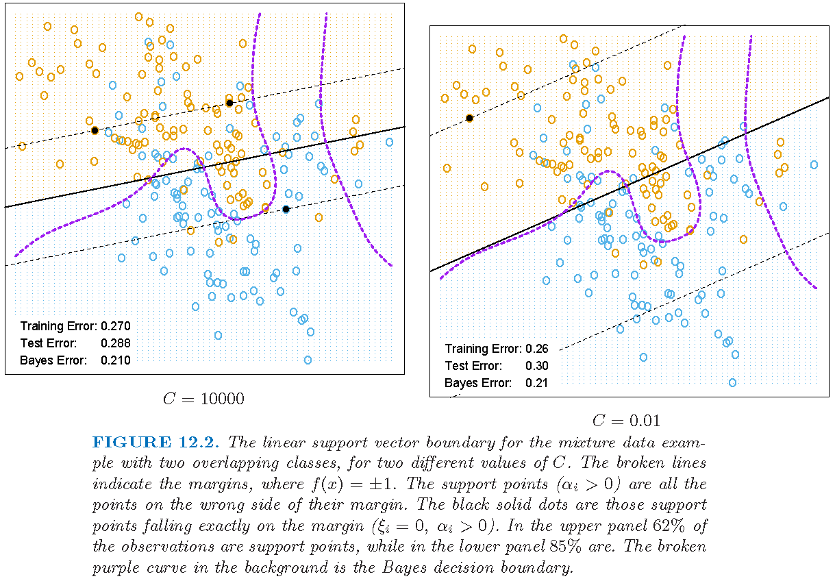
Margin and support vectors

Figure 12.2 of Supplementary Text (\(\alpha_i=a_i,\xi_i=\epsilon_i\)); \(C\) is the cost (smaller \(C\), wider margin):

License and session Information

License

> sessionInfo()
R version 3.5.0 (2018-04-23)
Platform: x86_64-w64-mingw32/x64 (64-bit)
Running under: Windows 10 x64 (build 19041)

Matrix products: default

locale:
[1] LC_COLLATE=English_United States.1252 
[2] LC_CTYPE=English_United States.1252   
[3] LC_MONETARY=English_United States.1252
[4] LC_NUMERIC=C                          
[5] LC_TIME=English_United States.1252    

attached base packages:
[1] stats     graphics  grDevices utils     datasets  methods  
[7] base     

other attached packages:
[1] plot3D_1.3 knitr_1.21

loaded via a namespace (and not attached):
 [1] compiler_3.5.0  magrittr_1.5    tools_3.5.0    
 [4] htmltools_0.3.6 misc3d_0.9-0    revealjs_0.9   
 [7] yaml_2.2.0      Rcpp_1.0.0      stringi_1.2.4  
[10] rmarkdown_1.11  stringr_1.3.1   xfun_0.4       
[13] digest_0.6.18   evaluate_0.12   tcltk_3.5.0