Stat 437 Lecture Notes 6a
Xiongzhi Chen
Washington State University

Support vector machines (SVMs)
Nonlinear decision boundary
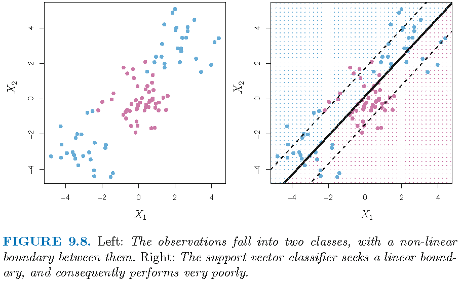
Need of a classifier with nonlinear decision boundary:
Enlarged feature space
Let us call a “linear classifier” a classifier with a linear decision boundary in the original feature space. One way to build a “nonlinear classifier” is
- to enlarge the original feature space by including nonlinearly transformed feature variables
- to apply a linear classifier, such as the support vector classifier (SVC) that is defined via the Euclidean inner product, to all feature variables in the enlarged feature space
This will give a decision boundary that is linear in the enlarged feature space but is nonlinear in the original feature space
SVC in enlarged feature space
We can build a support vector classifier (SVC) in an enlarged feature space as follows:
original feature space of dimension \(p\), generated by components of feature vector \(X=(X_1,\ldots,X_p)^T\)
enlarged feature space of dimension \(2p\), generated by components of \(X\) and of \(X^{\cdot 2}=(X_1^2,\ldots,X_p^2)^T\)
let \(x_i\) and \(x^{\cdot 2}{_{i}}\) be the \(i\)th observation for \(X\) and \(X^{\cdot 2}\), respectively
let \(y_i\) be the class label for \(x_i\)
SVC in enlarged feature space
- find optimal hyperplane \(\hat{S}=\hat{S}(\hat{\alpha}_1,\hat{\alpha}_2,\hat{\beta}_0)\) in the enlarged feature space by solving \[ \max\{M: \beta_{0} \in \mathbb{R}, \alpha_1, \alpha_2 \in \mathbb{R}^p, \Vert (\alpha_1^T,\alpha_2^T)^T \Vert =1\} \] subject to \[ \begin{aligned} & \forall i, y_{i}\left( \langle x_{i}, \alpha_1 \rangle + \langle x^{\cdot 2}{_{i}}, \alpha_2 \rangle +\beta_{0}\right) \geq M\left( 1-\epsilon_{i}\right)\\ & \quad \quad \epsilon_{i}\geq 0; \sum\nolimits_{i=1}^n\epsilon_{i}\leq C \text{ for some } C>0 \\ \end{aligned} \]
- the direction of \(\hat{S}\) is \[\hat{\alpha}=(\alpha_1^T,\alpha_2^T)^T \in \mathbb{R}^{2p}\]
- the SVC induced by \(\hat{S}\) assigns \((x_0^T,(x^{\cdot 2}{_{0}})^T)^T\) to class \[ \hat{y}_0 = \operatorname{sgn}( \langle x_{0}, \hat{\alpha}_1 \rangle + \langle x^{\cdot 2}{_{0}}, \hat{\alpha}_2 \rangle +\hat{\beta}_{0} ) \]
Enlarged feature space
The original feature space of dimension \(p\), generated by components of feature vector \(X=(X_1,\ldots,X_p)^T\), can be enlarged in different ways
However, enlarging original feature space may lead to unmanageable computations in the optimization problem that gives the corresponding classifier, if too many transforms of feature variables are incorporated
We need a sufficiently versatile and computationally efficient way to enlarge a feature space, and one such is the support vector machine (SVM)
SVM in a nutshell
Support vector classifier (SVC) uses the Euclidean inner product on the feature space and solves the optimization problem to obtain the optimal hyperplane and its induced classifier
Support vector machine (SVM) replaces the Euclidean inner product on the feature space by a kernel and solves the same type of optimizatin problem to obtain an optimal hypersurface and its induced classifier, yielding a nonlinear decision boundary in the original feature space when needed
Inner product
An inner product on \(\mathbb{R}^p \times \mathbb{R}^p\) is a bivariate function \(H\) of two vectors that is, for \(\lambda,\gamma,r,s \in \mathbb{R}\) and \(\mathbf{a},\mathbf{b},\mathbf{c},\mathbf{d} \in \mathbb{R}^p\),
- symmetric, i.e., \(H(\mathbf{a},\mathbf{b}) = H(\mathbf{b},\mathbf{a})\)
bi-linear, i.e., linearity in each argument, i.e., \[ \begin{aligned} & H(\lambda \mathbf{a} + \gamma \mathbf{c}, r \mathbf{b} + s \mathbf{d}) \\ = & \lambda r H( \mathbf{a}, \mathbf{b}) + \lambda s H( \mathbf{a}, \mathbf{d}) + \gamma r H(\mathbf{c}, \mathbf{b}) + \gamma s H(\mathbf{c}, \mathbf{d}) \end{aligned} \]
positive definite, i.e., \(H( \mathbf{a},\mathbf{a}) >0\) unless \(\mathbf{a}=0\)
The Euclidean inner product \(\langle \mathbf{a},\mathbf{b}\rangle = \sum_{i=1}^p a_i b_i\) for \(\mathbf{a}=(a_1,\ldots,a_p)^T,\mathbf{b}=(b_1,\ldots,b_p)^T \in \mathbb{R}^p\) is just one inner product among many inner products
Linear representation of SVC
For a support vector classifier (SVC), its optimal hyperplane \(\hat{S}=\hat{S}(\hat{\alpha},\hat{\beta}_0)\) has \(\hat{\alpha}=\sum_{i=1}^n \hat{a}_i y_i x_i\). Since Euclidean inner product \(\langle \cdot,\cdot\rangle\) is symmetric and bi-linear, we see \[ \langle x, \hat{\alpha} \rangle + \hat{\beta}_0 = \sum_{i=1}^n \hat{a}_i y_i \langle x,x_i \rangle + \hat{\beta}_0 \]
Let \[f(x; \hat{\alpha},\hat{\beta_0}) = \sum_{i=1}^n \hat{a}_i y_i \langle x,x_i \rangle + \hat{\beta}_0\] Then \(\hat{S}\) is the solution in \(x \in \mathbb{R}^p\) to \(f(x; \hat{\alpha},\hat{\beta_0})=0\), and \(f\) is called a linear representation for the SVC induced by \(\hat{S}\)
Support vector machines
- If we replace Euclidean inner product \(\langle \cdot,\cdot\rangle\) in the linear representation for SVC as \[f(x; \hat{\alpha},\hat{\beta_0}) = \sum_{i=1}^n \hat{a}_i y_i \langle x,x_i \rangle + \hat{\beta}_0\] by a symmetric, positive definite, bivariate function \(K(\cdot,\cdot)\) called a kernel, then we obtain a generalization \[ f_K(x; \hat{\alpha},\hat{\beta_0}) = \sum_{i=1}^n \hat{a}_i y_i K(x,x_i) + \hat{\beta}_0 \]
- The resulting classifier that assigns \(x_0\) to class \[ \hat{y}_0 = \operatorname*{sgn}(f_K(x_0; \hat{\alpha},\hat{\beta_0})) \] is called a support vector machine (SVM)
Some kernels
For \(\mathbf{a},\mathbf{b} \in \mathbb{R}^p\), some kernels include:
- Euclidean inner product \(K(\mathbf{a},\mathbf{b})=\langle \mathbf{a},\mathbf{b}\rangle\), which is called a linear kernel and gives the support vector classifier(SVC)
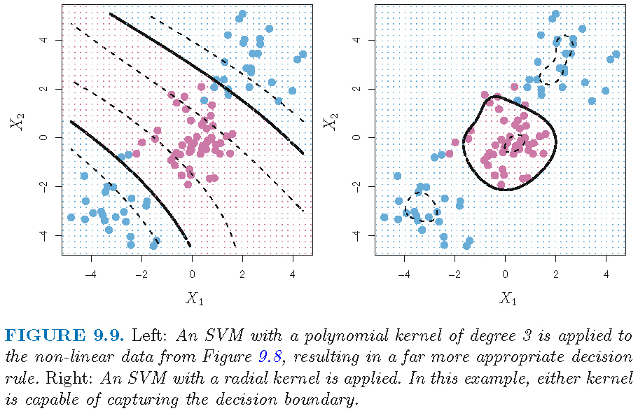
- Polynomial kernel of degree \(d \ge 1\) as \[K(\mathbf{a},\mathbf{b})= (1+ \langle \mathbf{a},\mathbf{b}\rangle)^d\] When \(d=1\), the resulting classifier is the SVC
- Radial kernel as \[ K(\mathbf{a},\mathbf{b})= \exp(-\gamma \Vert \mathbf{a} -\mathbf{b} \Vert^2) \text{ for some } \gamma >0, \] where \(\Vert \mathbf{a} -\mathbf{b} \Vert=d_{\mathbb{R}^p}(\mathbf{a},\mathbf{b})\) is Euclidean distance. For a new observation \(x_0\), \(K(x_0,x_i)\) is small when \(d_{\mathbb{R}^p}(x_0,x_i)\) is large. So, only nearby observations to \(x_0\) affect the predicted class label for \(x_0\)
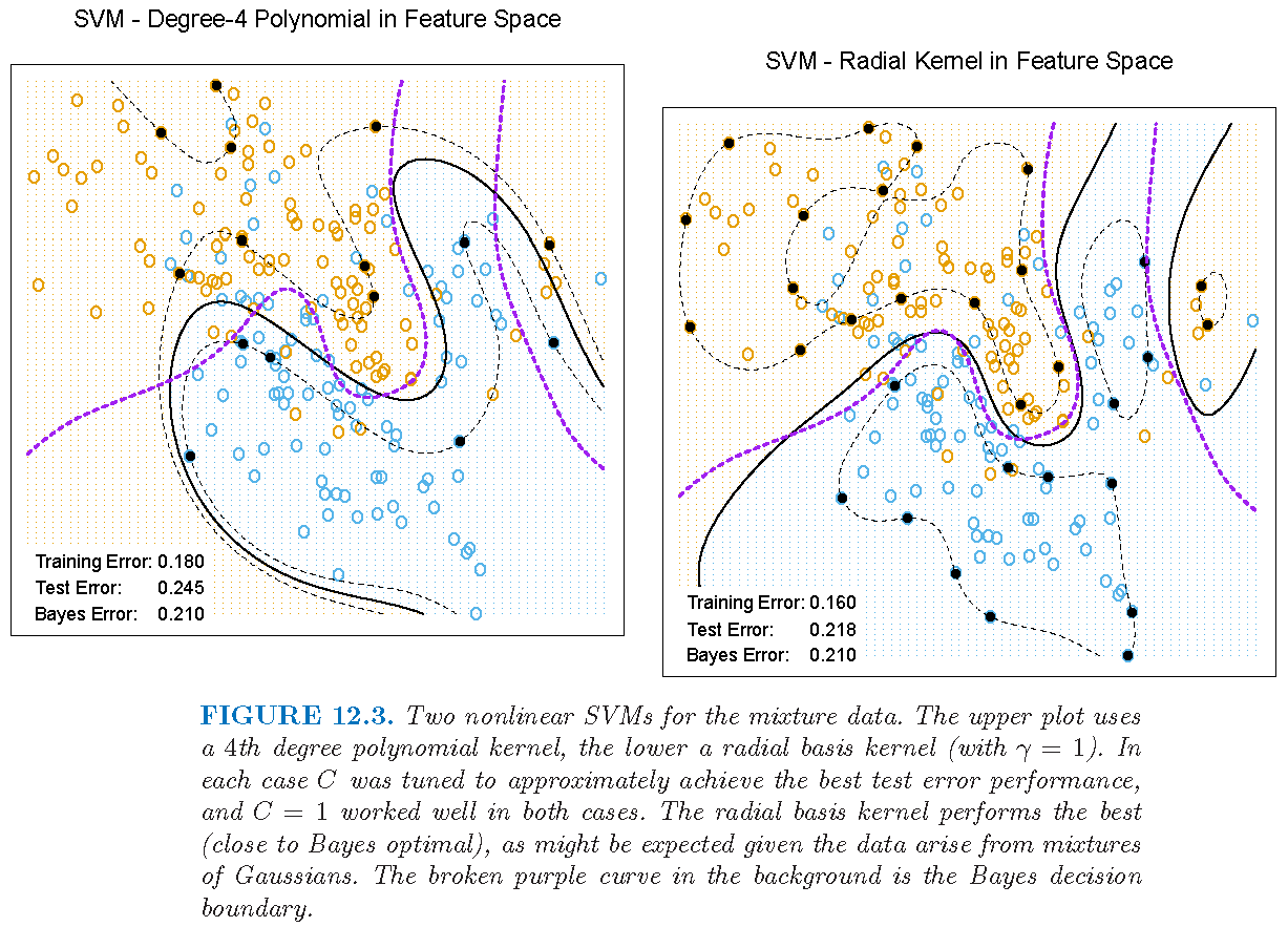
SVM with different kernels
SVM with different kernels
Figure 12.3 of Supplementary Text:
Advantages of kernels
In essence, an SVM implicitly enlarges the feature space via the use of a kernel
One advantage of using a kernel over explicitly enlarging feature space is that we need only compute \(K(x_i,x_{i'})\) for all \(\binom{n}{2}\) distinct pairs \((i,i')\), without explicitly working in the enlarged feature space
This is important because in many applications of SVMs, the enlarged feature space can be so large that computations are intractable
Optimization for SVM
From Chapter 12 of Supplementary Text, we see that an SVM maximizes the “Lagrange dual function” \[ L_{D} = \sum_{i=1}^n a_{i} - 2^{-1}\sum_{i=1}^n \sum_{i'=1}^n a_{i} a_{i'}y_{i} y_{i'} K( x_i, x_{i'}) \] with constraint \(\sum_{i=1}^n a_i y_i =0\) and \(0 \le a_i \le C\)
In the optimal solution \[ f_K(x; \hat{\alpha},\hat{\beta_0}) = \sum_{i=1}^n \hat{a}_i y_i K(x,x_i) + \hat{\beta}_0, \] an \(x_i\) such that \(\hat{a}_i \ne 0\) is a support vector
SVM application: data set
Heartdata: 13 features such asAge,SexandChol(serum cholestoral in mg/dl), and \(303\) observations- Target: to predict whether an individual has heart disease, i.e.,
AHD=YesorAHD=No
  Age Sex Chol AHD
1  63   1  233  No
2  67   1  286 Yes
3 67 1 229 Yes- LDA and SVC compute scores of the form \[\hat{f}(X)=\hat{\beta}_0 + \langle X,\hat{\alpha} \rangle\]
- For any cutoff \(t\), \(X\) is classified into
AHD=YesorAHD=Nodepending on whether \(\hat{f}(X)<t\) or \(\hat{f}(X) \ge t\)
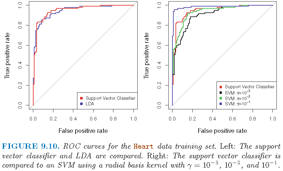
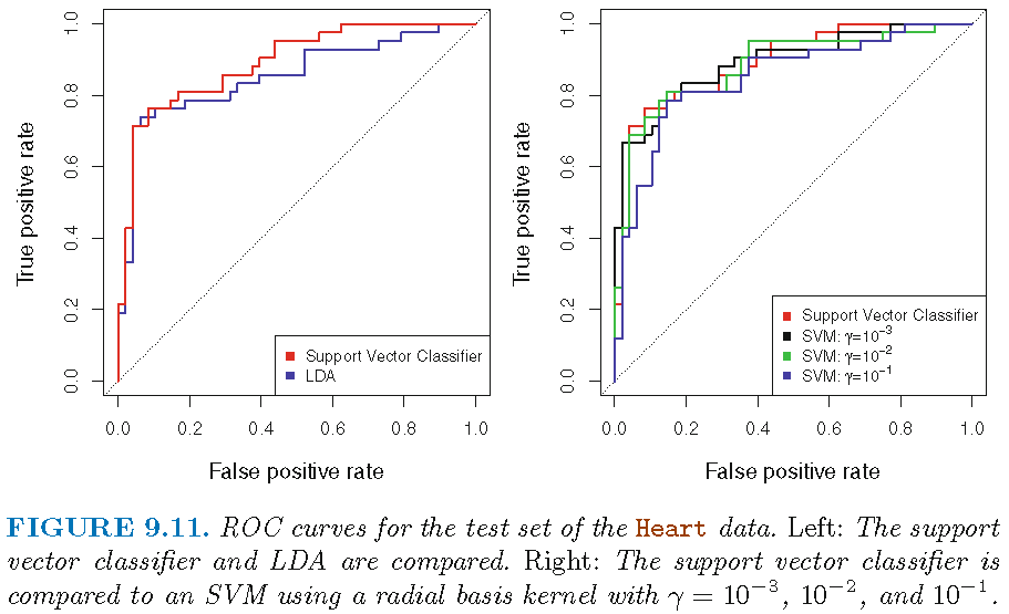
SVM: ROC curve on training set
SVC seems to be better than LDA; SVM with \(\gamma=0.1\) radial kernel seems to give perfect ROC curve
SVM: ROC curve on test set
90 test observations; SVC seems to be better than LDA; SVM with \(\gamma=0.1\) radial kernel seems to be worst
Support vector machine: miscellaneous
SVM for multiclass settings
When there are \(s>2\) classes, we can do either
- One-versus-One classification approach: construct \(\binom{s}{2}\) SVMs, each of which compares a pair of classes. A test observation \(x_0\) is assigned to the class to which \(x_0\) is the mostly frequently assigned by the \(\binom{s}{2}\) SVMs
- One-versus-All classification approach: construct \(s\) SVMs as \[ f_{K,r}(x; \hat{\alpha}_r,\hat{\beta}_{r0}) = \sum_{i=1}^n \hat{a}_{ri} y_i K(x,x_i) + \hat{\beta}_{r0}, r=1,\ldots,s, \] each of which compares one of the \(s\) classes with the remaining \(s-1\) classes. \(x_0\) is assigned to class \[ \tilde{k}=\operatorname{argmax}_{1\le k \le s} f_{K,k}(x_0;\hat{\alpha}_k,\hat{\beta}_{k0}) \]
SVM and hinge loss
Recall the linear representation for support vector classifier (SVC) \[f(x; {\beta}, {\beta_0}) = \langle x, \beta \rangle + {\beta}_0\] with \(\beta=(\beta_1,\ldots,\beta_p)^T\)
The optimization problem that produces SVC is equivalent to \[ \min_{\beta_0 \in \mathbb{R},\alpha \in \mathbb{R}^p} \left\{ \overbrace{\sum_{i=1}^n \underbrace{\max[0,1-y_i f(x_i; {\beta}, {\beta_0})]}_{\text{hinge loss}}}^{\text{empirical loss } L(\mathbf{X},\mathbf{y})} + \overbrace{\underbrace{\lambda \Vert \beta \Vert^2}_{\text{ridge penalty}}}^{\text{penalty } P(\beta)} \right\} \]
Hinge loss and logistic regression
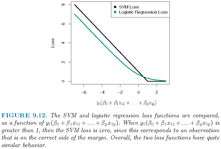
SVM and logistic regression
The hinge loss \(l(t)=\max(0,1-t)\) is zero if \(t \ge 1\), i.e., the loss is zero if \[y_i(\langle x_i, \beta \rangle + {\beta}_0) \ge 1,\] i.e., if \(x_i\) is on the correct side of the margin
But the loss function for logistic regression is not exactly zero anywhere, and it is very small for observations that are far from the decision boundary
Hence, logistic regression and SVMs often give very similar results. When the classes are well separated, SVMs tend to behave better than logistic regression; in more overlapping regimes, logistic regression is often preferred
License and session Information
> sessionInfo()
R version 3.5.0 (2018-04-23)
Platform: x86_64-w64-mingw32/x64 (64-bit)
Running under: Windows 10 x64 (build 19041)

Matrix products: default

locale:
[1] LC_COLLATE=English_United States.1252
[2] LC_CTYPE=English_United States.1252
[3] LC_MONETARY=English_United States.1252
[4] LC_NUMERIC=C
[5] LC_TIME=English_United States.1252

attached base packages:
[1] stats     graphics  grDevices utils     datasets  methods
[7] base

other attached packages:
[1] knitr_1.21

loaded via a namespace (and not attached):
 [1] compiler_3.5.0  magrittr_1.5    tools_3.5.0
 [4] htmltools_0.3.6 revealjs_0.9    yaml_2.2.0
 [7] Rcpp_1.0.0      stringi_1.2.4   rmarkdown_1.11
[10] stringr_1.3.1   xfun_0.4        digest_0.6.18
[13] evaluate_0.12