Stat 437 Lecture Notes 6b

Xiongzhi Chen

Washington State University

Support vector machines: software implementation

R software and commands

R libraries and commands needed:

R library e1071, command svm{e1071} to construct a support vector machine (SVM), and command tune{e1071} to determine cost parameter $C$ (and kernel parameters) by cross-validation
R library LiblineaR for very large linear problems (not discussed here)

Command `svm{e1071}`

svm{e1071} is used to train a support vector machine. Its basic syntax is

svm(formula, data=NULL, subset, scale=TRUE, kernel="radial",
     degree=3, gamma=if (is.vector(x)) 1 else 1/ncol(x),
     cost=1, na.action=na.omit, ...)

formula: a symbolic description of the model to be fit.
data: an optional data frame containing the variables in the model. By default the variables are taken from the environment which svm is called from.
subset: an index vector specifying the cases to be used in the training sample. (NOTE: If given, this argument must be named.)

Command `svm{e1071}`

Basic syntax:

svm(formula, data=NULL, subset, scale=TRUE, kernel="radial",
     degree=3, gamma=if (is.vector(x)) 1 else 1/ncol(x),
     cost=1, na.action=na.omit, ...)

scale: a logical vector indicating the variables to be scaled. By default, data are scaled internally (both x and y variables) to zero mean and unit variance. The center and scale values are returned and used for later predictions.
kernel: the kernel used in training and predicting, which can be linear (i.e., the Euclidean inner product), polynomial with degree, or radial (i.e., the radial kernel).

Command `svm{e1071}`

Basic syntax:

svm(formula, data=NULL, subset, scale=TRUE, kernel="radial",
     degree=3, gamma=if (is.vector(x)) 1 else 1/ncol(x),
     cost=1, na.action=na.omit, ...)

degree: degree of polynomial kernel; default is 3.
gamma: parameter needed for radial kernel; default is $1/p$ (where $p$ is the number of features).
cost: cost of constraints on violation, i.e., the cost $C$ in the Lagrange multiplier function; default is 1.

Command `svm{e1071}`

svm{e1071} returns an object of class svm containing the fitted model, including:

SV: support vectors (possibly scaled).
index: indices of support vectors in the data matrix. Note that this index refers to the preprocessed data (after the possible effect of na.omit and subset).
coefs: coefficients (i.e., entries of the direction vector of optimal hyperplane) times the training labels.
rho: the negative intercept (of optimal hyperplane).

Command `tune{e1071}`

tune{e1071} tunes hyperparameters of statistical methods using a grid search over supplied parameter ranges. Its basic syntax is:

tune(method, data = list(), ranges = NULL, ...)

method: either the function to be tuned, or a character string naming such a function.
data: data, if a formula interface is used; ignored, if predictor matrix and response are supplied directly.
ranges: a named list of parameter vectors spanning the sampling space. The vectors will usually be created by seq.

Command `tune{e1071}`

Basic syntax:

tune(method, data = list(), ranges = NULL, ...)

...: additional parameters and some parameters of method

tune{e1071} returns an object of class tune, including the components:

best.parameters: a 1 x k data frame with k as number of parameters.
best.performance: best achieved performance.

Support vector classifier (SVC): Example 1a

Nonseparable data

Generate nonseparable data:

$n=20$ observations on $p=2$ features $X_1,X_2$
Class $-1$: $x_i \sim \text{Gaussian}(\mu_1=(0,0)^T,\mathbf{I}),i=1,\ldots,10$
Class $1$: $x_i \sim \text{Gaussian}(\mu_2=(1,1)^T,\mathbf{I}),i=11,\ldots,20$

> set.seed(1)
> x=matrix(rnorm(20*2), ncol=2)
> y=c(rep(-1,10), rep(1,10))
> x[y==1,]=x[y==1,] + 1
> dat=data.frame(x=x, y=as.factor(y))

Scatter plot

No separating hyperplane:

> par(mar = c(4.9, 4.5, .0, .5),oma=c(1.3,1.3,0.3,1.3))
> plot(x,col=(3-y),xlab=expression(X[1]),ylab=expression(X[2]))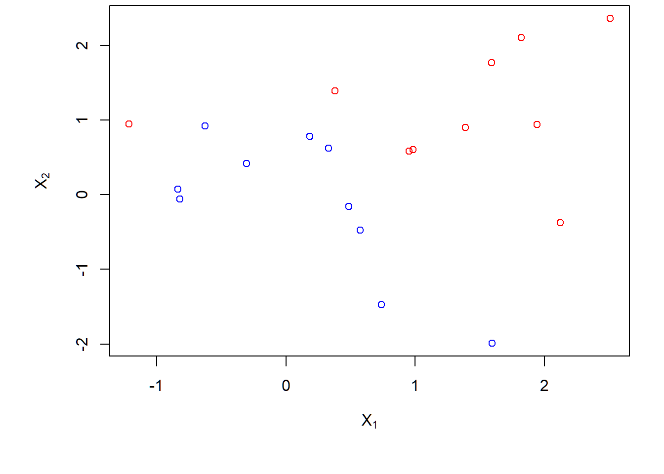

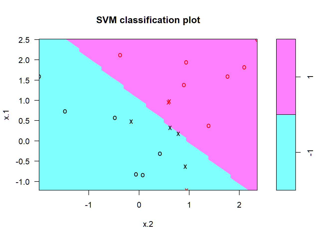
SVC: $C=10$

SVC with cost $C=10$:

> library(e1071)
> svmfit=svm(y~.,data=dat,kernel="linear",cost=10,scale=FALSE)
> svmfit$index # indices of support vectors
> summary(svmfit)
> plot(svmfit, dat) # X_2 on x-axis

scale as TRUE or FALSE dependent on scales of measurements on feature variables
summary(svm.ojb): provide a summary of model and results
plot(svm.ojb,data): create visualization of classification results by plotting 2nd feature on x-axis

SVC: $C=10$

Summary of model fit:

[1]  1  2  5  7 14 16 17

Call:
svm(formula = y ~ ., data = dat, kernel = "linear", 
    cost = 10, scale = FALSE)


Parameters:
   SVM-Type:  C-classification 
 SVM-Kernel:  linear 
       cost:  10 
      gamma:  0.5 

Number of Support Vectors:  7

 ( 4 3 )


Number of Classes:  2 

Levels: 
 -1 1

4 support vectors in one class and 3 in the other

SVC: $C=10$

Support vectors as crosses; others observations as circles

SVC: $C=0.1$

> svmfit=svm(y~.,data=dat,kernel="linear",cost=0.1,scale=FALSE)
> svmfit$index
 [1]  1  2  3  4  5  7  9 10 12 13 14 15 16 17 18 20
> par(mar = c(4.9, 4.5, 1.8, .5),oma=c(1.3,1.3,0.3,1.3)); plot(svmfit, dat)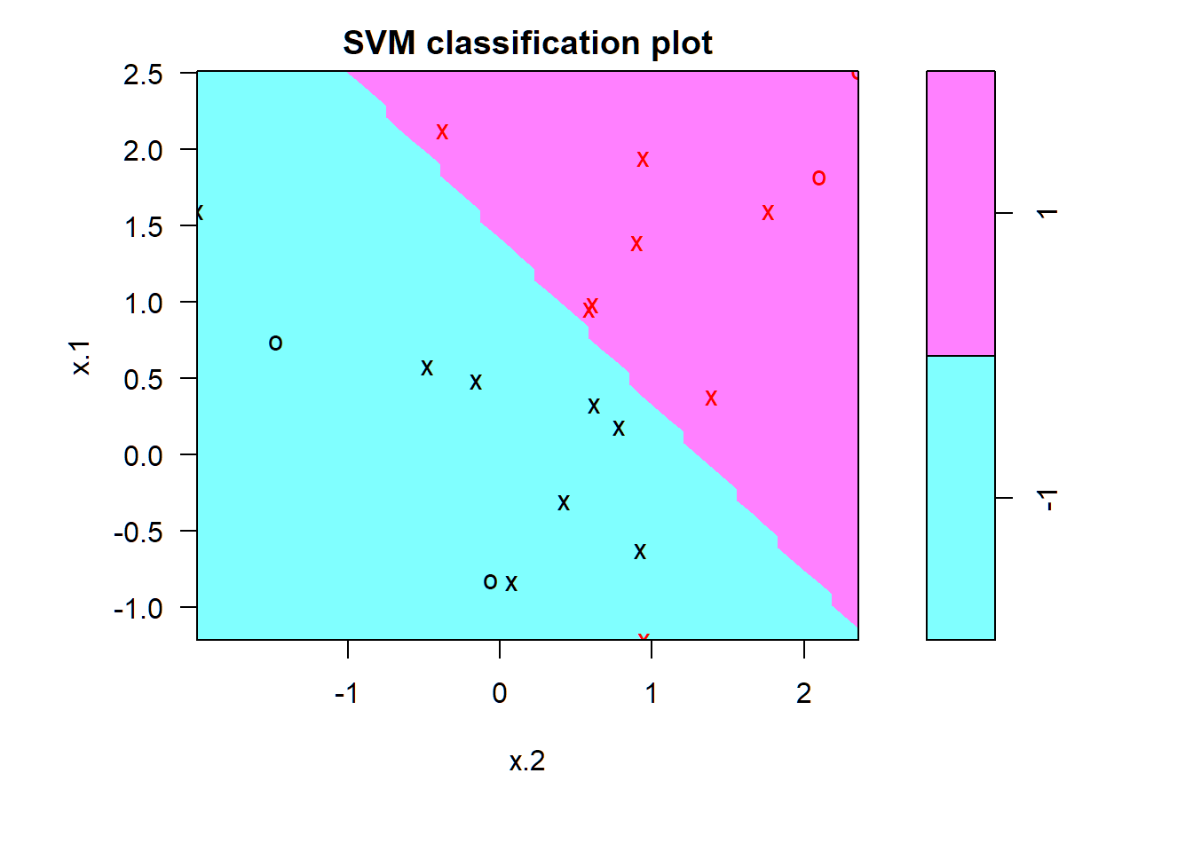

Cross-validation on $C$

> set.seed(1)
> tune.out=tune(svm,y~.,data=dat,kernel="linear",
+           ranges=list(cost=c(0.001, 0.01, 0.1, 1,5,10,100)))
> summary(tune.out)

Parameter tuning of 'svm':

- sampling method: 10-fold cross validation 

- best parameters:
 cost
  0.1

- best performance: 0.1 

- Detailed performance results:
   cost error dispersion
1 1e-03  0.70  0.4216370
2 1e-02  0.70  0.4216370
3 1e-01  0.10  0.2108185
4 1e+00  0.15  0.2415229
5 5e+00  0.15  0.2415229
6 1e+01  0.15  0.2415229
7 1e+02  0.15  0.2415229

set.seed needed since cross-validation randomly divides data into splits of approximately equal size

Obtain best model

Obtain best model given by cross-validation: $C=0.1$

> bestmod=tune.out$best.model
> summary(bestmod)

Call:
best.tune(method = svm, train.x = y ~ ., data = dat, 
    ranges = list(cost = c(0.001, 0.01, 0.1, 1, 5, 
        10, 100)), kernel = "linear")


Parameters:
   SVM-Type:  C-classification 
 SVM-Kernel:  linear 
       cost:  0.1 
      gamma:  0.5 

Number of Support Vectors:  16

 ( 8 8 )


Number of Classes:  2 

Levels: 
 -1 1

tune.obj$best.model: best model given by cross-validation

Best model applied to test set

Generate test set:

$n=20$ observations on $p=2$ features $X_1,X_2$
Class $-1$: $x_i \sim \text{Gaussian}(\mu_1=(0,0)^T,\mathbf{I})$
Class $1$: $x_j \sim \text{Gaussian}(\mu_2=(1,1)^T,\mathbf{I})$

> set.seed(1)
> xtest=matrix(rnorm(20*2), ncol=2)
> # create class labels
> ytest=sample(c(-1,1), 20, rep=TRUE)
> xtest[ytest==1,]=xtest[ytest==1,] + 1
> testdat=data.frame(x=xtest, y=as.factor(ytest))
> ypred=predict(bestmod,testdat)
> table(predict=ypred, truth=testdat$y)
       truth
predict -1  1
     -1 10  1
     1   1  8

note the syntax predict(svm.ojb,data)

SVC: $C=0.01$

SVC with $C=0.01$ on training data:

> svmfit=svm(y~.,data=dat,kernel="linear",cost=.01,scale=FALSE)
> ypred1=predict(svmfit,testdat)
> table(predict=ypred1, truth=testdat$y)
       truth
predict -1  1
     -1 10  4
     1   1  5

Caution: not able to reproduce Text results for this
$C=0.01$ not as good as $C=0.1$

Support vector classifier (SVC): Example 1b

Barely separable data

Observations barely separable by a hyperplane:

> x[y==1,]=x[y==1,]+0.5; dat=data.frame(x=x,y=as.factor(y))
> par(mar=c(6.2,4.5,.0,.5),oma=c(1.3,1.3,0.3,1.3))
> plot(x, col=(y+5)/2, pch=19,
+      xlab=expression(X[1]),ylab=expression(X[2]))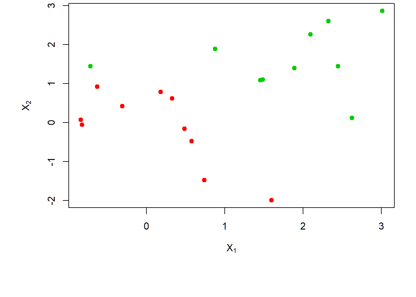

SVC: $C=10^{5}$

SVC with cost $C=10^{5}$:

> svmfit=svm(y~., data=dat, kernel="linear", cost=1e5)
> summary(svmfit)

Call:
svm(formula = y ~ ., data = dat, kernel = "linear", 
    cost = 1e+05)


Parameters:
   SVM-Type:  C-classification 
 SVM-Kernel:  linear 
       cost:  1e+05 
      gamma:  0.5 

Number of Support Vectors:  3

 ( 1 2 )


Number of Classes:  2 

Levels: 
 -1 1

$C$ very large so that no observations are misclassified

SVC: $C=10^{5}$

Zero training error; fitted model may overfit training set and not perform well on test set

> par(mar=c(7,4.5,1.2,.5),oma=c(1.3,1.3,0.3,1.3)); plot(svmfit, dat)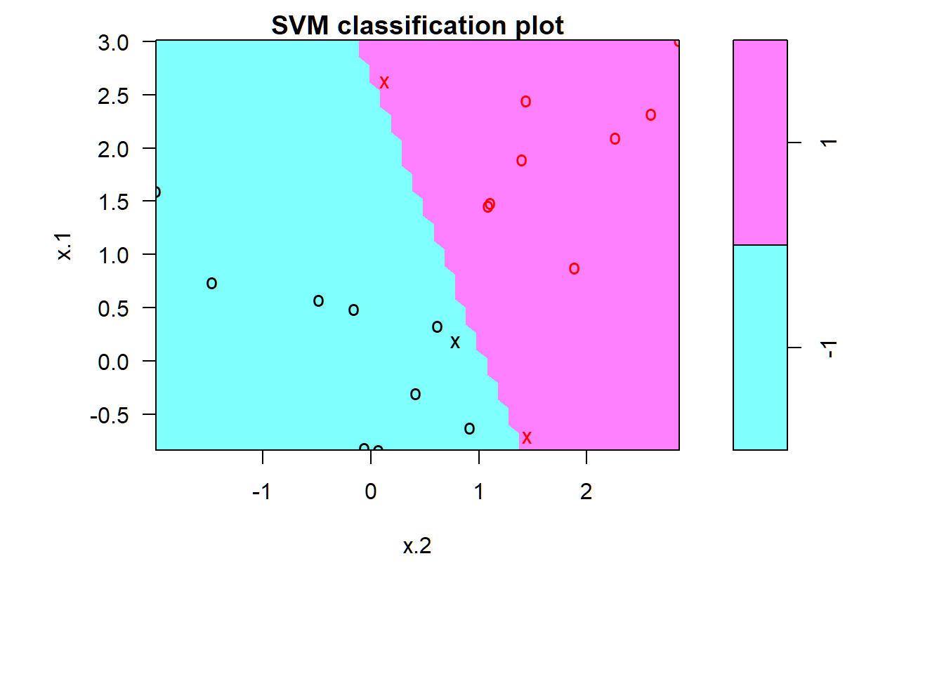

SVC: $C=1$

SVC with cost $C=1$:

> svmfit=svm(y~., data=dat, kernel="linear", cost=1)
> summary(svmfit)

Call:
svm(formula = y ~ ., data = dat, kernel = "linear", 
    cost = 1)


Parameters:
   SVM-Type:  C-classification 
 SVM-Kernel:  linear 
       cost:  1 
      gamma:  0.5 

Number of Support Vectors:  7

 ( 4 3 )


Number of Classes:  2 

Levels: 
 -1 1

SVC: $C=1$

1 observation misclassified; fitted model may perform well on test set

> par(mar=c(7,4.5,1.2,.5),oma=c(1.3,1.3,0.3,1.3)); plot(svmfit,dat)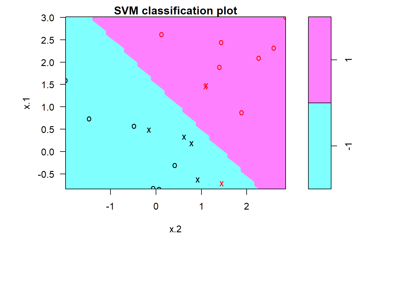

Support vector machines (SVMs): Example 1

Generate data

Data with a nonlinear class boundary:

$n=200$ observations on $p=2$ features $X_1,X_2$
Class $1$: $150$ observations; \[x_i \sim \text{Gaussian}(\mu_1=(2,2)^T,\mathbf{I}),i=1,\ldots,100\\ x_i \sim \text{Gaussian}(\mu_2=(-2,-2)^T,\mathbf{I}),i=101,\ldots,150 \]
Class $2$: $50$ observations; $x_i \sim \text{Gaussian}(\mu_3=(0,0)^T,\mathbf{I}),i=151,\ldots,200$

> set.seed(1)
> x=matrix(rnorm(200*2), ncol=2)
> x[1:100,]=x[1:100,]+2
> x[101:150,]=x[101:150,]-2
> y=c(rep(1,150),rep(2,50))
> dat=data.frame(x=x,y=as.factor(y))

Scatter plot

Data with a nonlinear class boundary:

> par(mar=c(7,4.5,1.2,.5),oma=c(1.3,1.3,0.3,1.3))
> plot(x, col=y,xlab=expression(X[1]),ylab=expression(X[2]))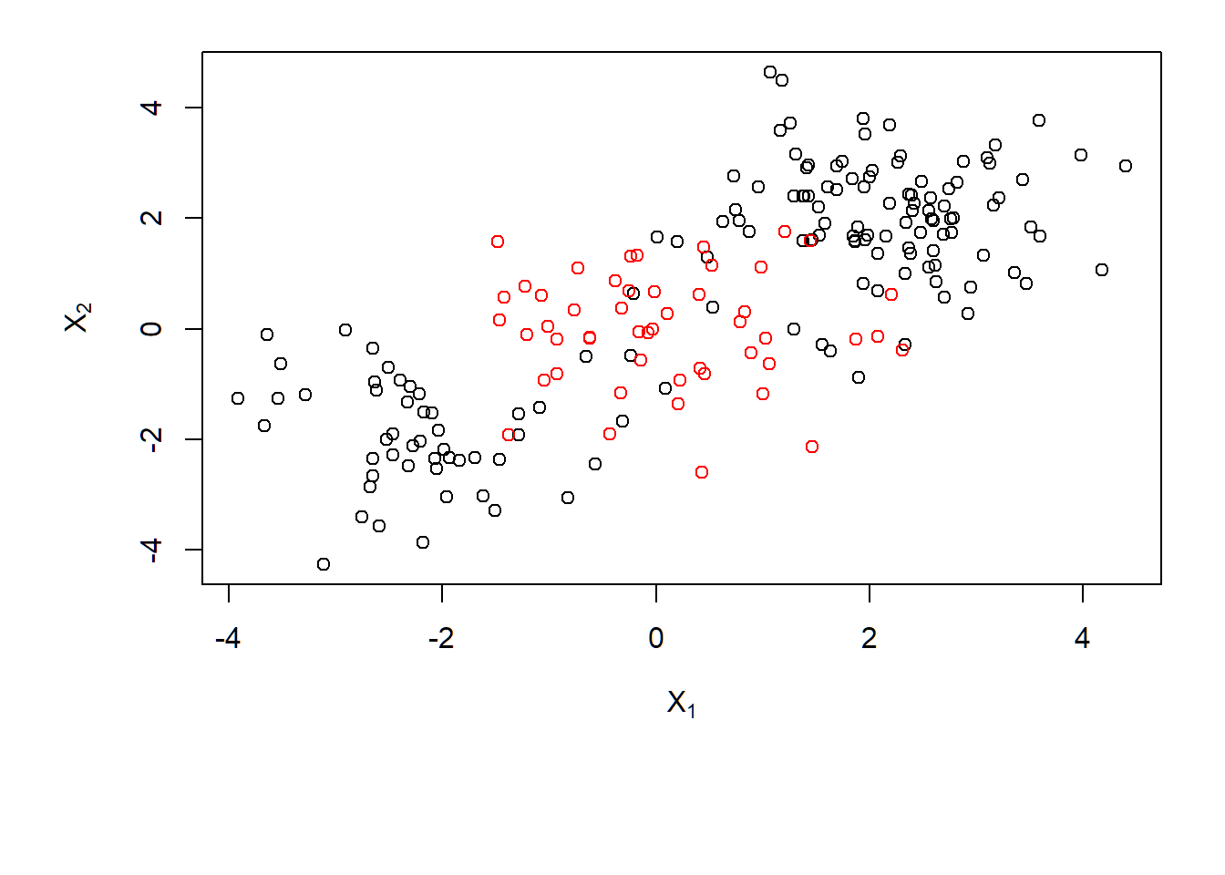

SVM: radial kernel; $C=1$

SVM with radial kernel and $\gamma=1$ and cost $C=1$ on training set of $100$ observations:

> train=sample(200,100) # training obs index
> svmfit=svm(y~., data=dat[train,], kernel="radial",
+            gamma=1, cost=1)
> summary(svmfit)

Call:
svm(formula = y ~ ., data = dat[train, ], kernel = "radial", 
    gamma = 1, cost = 1)


Parameters:
   SVM-Type:  C-classification 
 SVM-Kernel:  radial 
       cost:  1 
      gamma:  1 

Number of Support Vectors:  37

 ( 17 20 )


Number of Classes:  2 

Levels: 
 1 2

SVM: radial kernel; $C=1$

Support vectors as crosses; other observations as circles; fair number of training errors:

> par(mar=c(7,4.5,1.4,.5),oma=c(1.3,1.3,0.3,1.3)); plot(svmfit, dat[train,])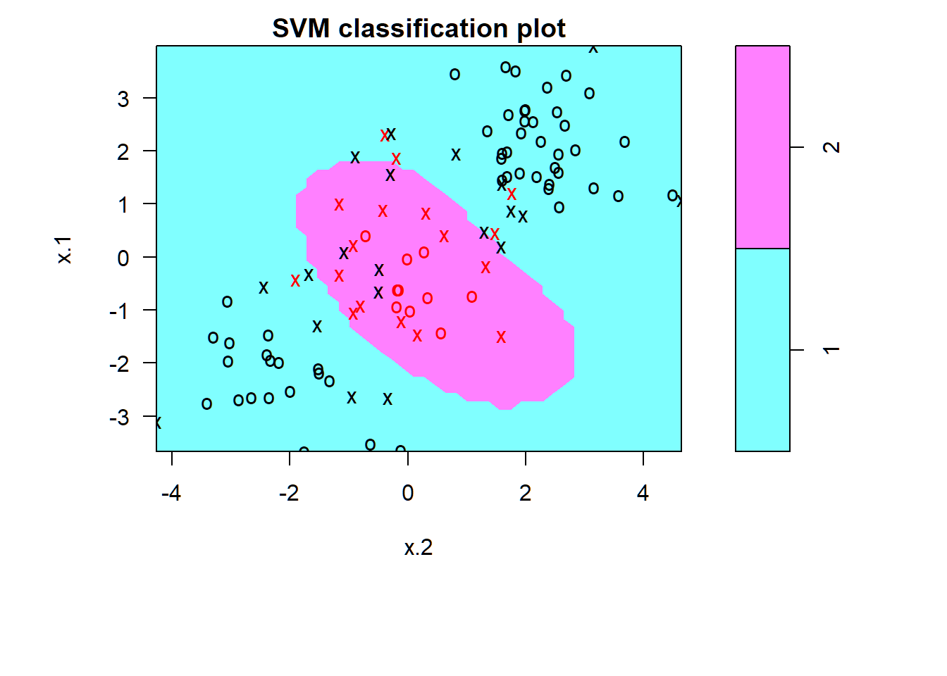

SVM: radial kernel; $C=10^5$

Less training error; risk of overfitting training data

> svmfit=svm(y~., data=dat[train,], kernel="radial",
+            gamma=1,cost=1e5)
> par(mar=c(7,4.5,1.4,.5),oma=c(1.3,1.3,0.3,1.3)); plot(svmfit,dat[train,])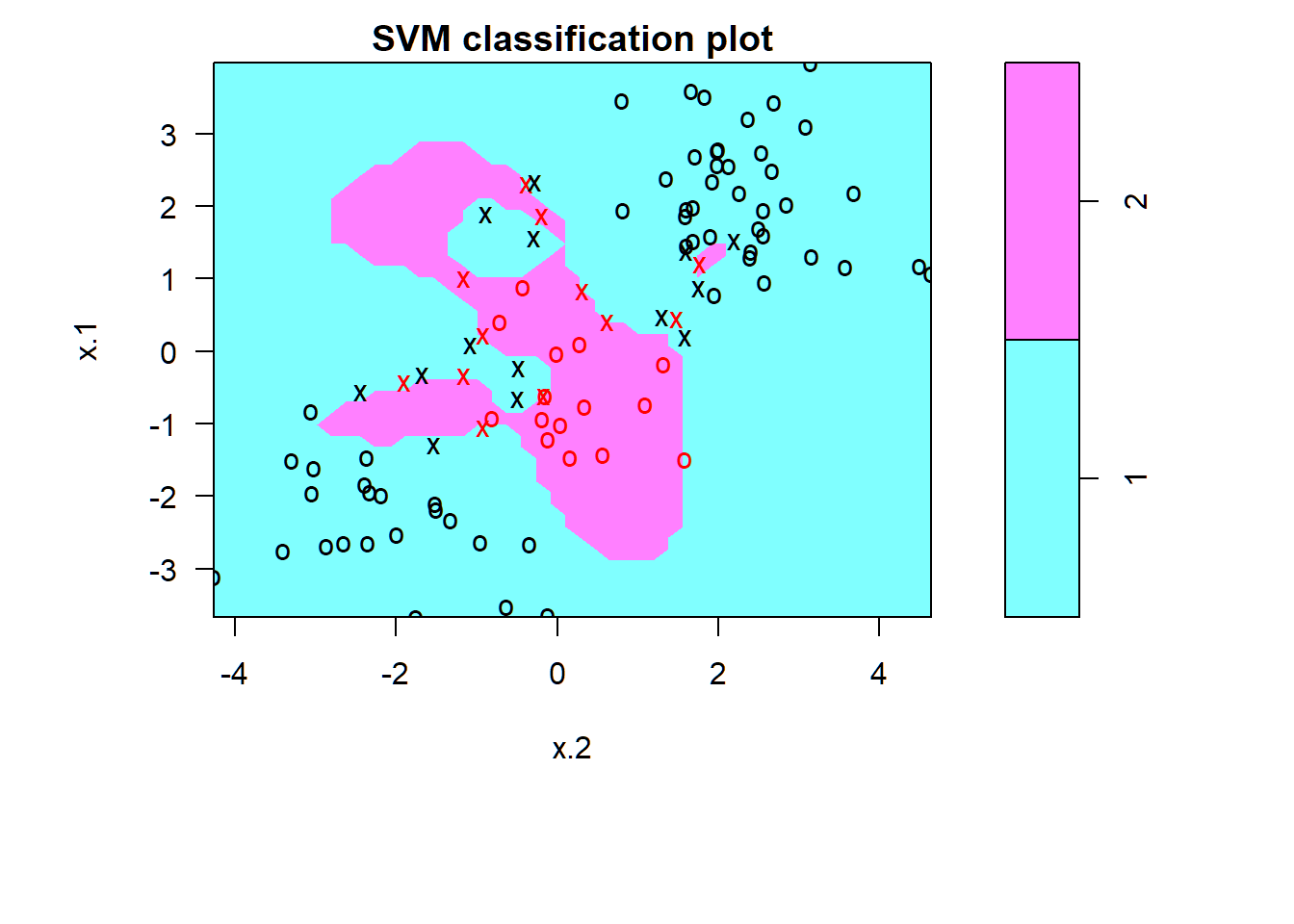

Cross-valiation on $C,\gamma$

Optimal parameter values determined by 10-fold cross-validation on training set: $C=1,\gamma=2$

> set.seed(1)
> tune.out=tune(svm, y~., data=dat[train,], kernel="radial", 
+               ranges=list(cost=c(0.1,1,10,100,1000),
+                           gamma=c(0.5,1,2,3,4)))
> summary(tune.out)

Parameter tuning of 'svm':

- sampling method: 10-fold cross validation 

- best parameters:
 cost gamma
    1     2

- best performance: 0.12 

- Detailed performance results:
    cost gamma error dispersion
1  1e-01   0.5  0.27 0.11595018
2  1e+00   0.5  0.13 0.08232726
3  1e+01   0.5  0.15 0.07071068
4  1e+02   0.5  0.17 0.08232726
5  1e+03   0.5  0.21 0.09944289
6  1e-01   1.0  0.25 0.13540064
7  1e+00   1.0  0.13 0.08232726
8  1e+01   1.0  0.16 0.06992059
9  1e+02   1.0  0.20 0.09428090
10 1e+03   1.0  0.20 0.08164966
11 1e-01   2.0  0.25 0.12692955
12 1e+00   2.0  0.12 0.09189366
13 1e+01   2.0  0.17 0.09486833
14 1e+02   2.0  0.19 0.09944289
15 1e+03   2.0  0.20 0.09428090
16 1e-01   3.0  0.27 0.11595018
17 1e+00   3.0  0.13 0.09486833
18 1e+01   3.0  0.18 0.10327956
19 1e+02   3.0  0.21 0.08755950
20 1e+03   3.0  0.22 0.10327956
21 1e-01   4.0  0.27 0.11595018
22 1e+00   4.0  0.15 0.10801234
23 1e+01   4.0  0.18 0.11352924
24 1e+02   4.0  0.21 0.08755950
25 1e+03   4.0  0.24 0.10749677
> table(true=dat[-train,"y"], 
+       pred=predict(tune.out$best.model,newdata=dat[-train,]))
    pred
true  1  2
   1 74  3
   2  7 16

ROC curve: function

Function to obtain ROC curve:

> library(ROCR)
> rocplot=function(pred, truth, ...){
+    predob = prediction(pred, truth)
+    perf = performance(predob, "tpr", "fpr")
+    plot(perf,...)}

Fitted values and ROC curves

> # apply optimal SVM to training set for prediction
> svmfit.opt=svm(y~., data=dat[train,], kernel="radial",
+                gamma=2, cost=1,decision.values=T)
> fitted=attributes(predict(svmfit.opt,dat[train,],
+                     decision.values=TRUE))$decision.values
> par(mfrow=c(1,2))
> rocplot(fitted,dat[train,"y"],main="Training Data")
> # another SVM built on training set and 
> # applied to it for prediction with gamma=50
> svmfit.flex=svm(y~., data=dat[train,], kernel="radial",
+                 gamma=50, cost=1, decision.values=T)
> fitted=attributes(predict(svmfit.flex,dat[train,],
+                   decision.values=T))$decision.values
> rocplot(fitted,dat[train,"y"],add=T,col="red")

decision.values: fitted value $f_K(x; \hat{\alpha},\hat{\beta_0}) = \sum_{i=1}^n \hat{a}_i y_i K(x,x_i) + \hat{\beta}_0$ for a value $x$ of feature vector $X$
attributes(predict.obj)$decision.values: $\hat{f}(x)$ when $x$ is a test observation

Fitted values and ROC curves

> # optimal model SVM applied to test set for prediction
> fitted=attributes(predict(svmfit.opt,dat[-train,],
+                   decision.values=T))$decision.values
> rocplot(fitted,dat[-train,"y"],main="Test Data")
> # non-optimal SVM applied to tet set for prediction
> fitted=attributes(predict(svmfit.flex,dat[-train,],
+                   decision.values=T))$decision.values
> rocplot(fitted,dat[-train,"y"],add=T,col="red")

“optimal” $\gamma=2$ obtained from range gamma=c(0.5,1,2,3,4) by 10-fold cross-validation on training set; so, another value for $\gamma$ may improve the “optimal” SVM on training set
another SVM is built with $\gamma=50$ and $C=1$ on training set

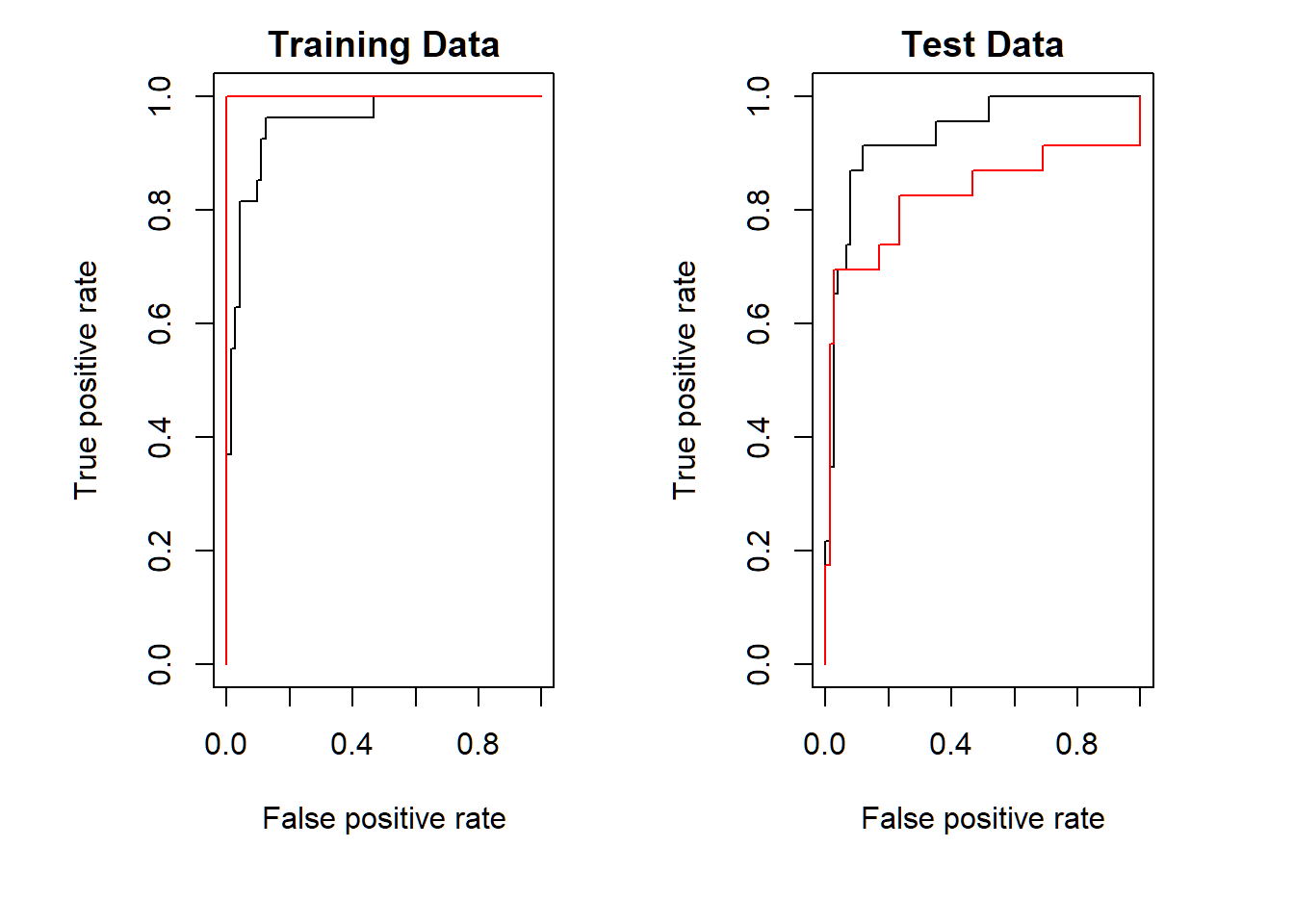
ROC curves: radial SVM

SVM with $\gamma=50,C=1$ (red) more accurate than SVM with $\gamma=2,C=1$ (black) on training set; the opposite happens on test set

Support vector machines (SVMs): Example 2

Generate data

$n=250$ observations on $p=2$ features $X_1,X_2$
Class $1$: $\quad 150$ observations; \[x_i \sim \text{Gaussian}(\mu_1=(2,2)^T,\mathbf{I}),i=1,\ldots,100\\ x_i \sim \text{Gaussian}(\mu_2=(-2,-2)^T,\mathbf{I}),i=101,\ldots,150 \]
Class $2$: $\quad 50$ observations; $x_i \sim \text{Gaussian}(\mu_3=(0,0)^T,\mathbf{I}),i=151,\ldots,200$
Class $0$: $\quad 50$ observations; $x_i \sim \text{Gaussian}(\mu_4=(0,2)^T,\mathbf{I}),i=201,\ldots,250$

> set.seed(1); x=matrix(rnorm(200*2),ncol=2)
> x[1:100,]=x[1:100,]+2; x[101:150,]=x[101:150,]-2
> y=c(rep(1,150),rep(2,50))
> x=rbind(x, matrix(rnorm(50*2), ncol=2))
> y=c(y, rep(0,50)); x[y==0,2]=x[y==0,2]+2
> dat=data.frame(x=x, y=as.factor(y))

Scatter plot

3 classes with nonlinear class boundary:

> par(mar=c(5.5,4.5,1.2,.5),oma=c(1.3,1.3,0.3,1.3))
> plot(x,col=(y+1),xlab=expression(X[1]),ylab=expression(X[2]))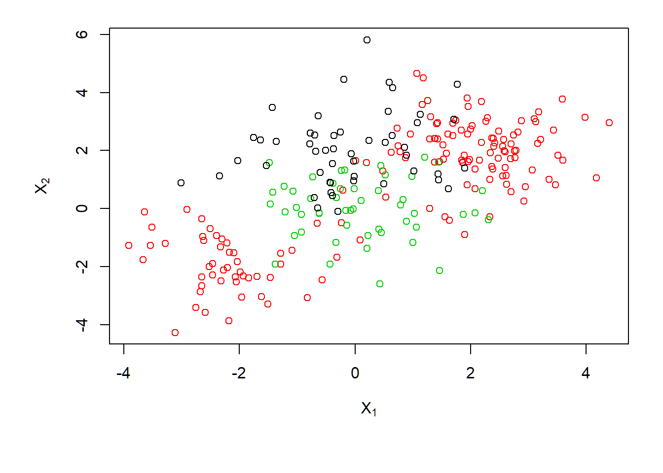

SVM with radial kernel

> svmfit=svm(y~., data=dat, kernel="radial", cost=10, gamma=1)
> plot(svmfit, dat)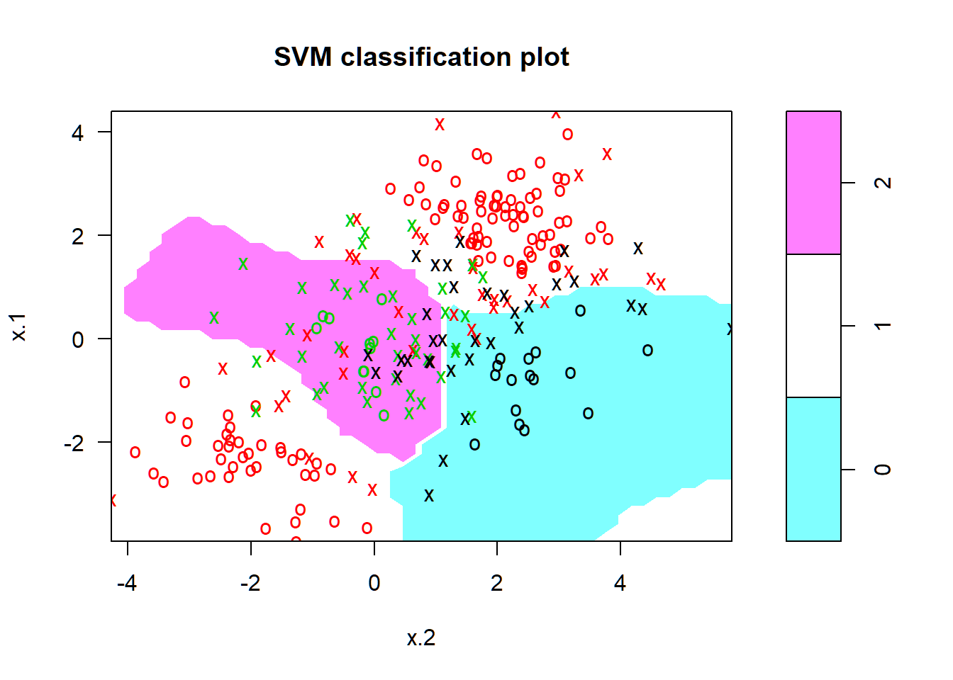

Support vector machines (SVMs): Example 3

Gene expression data

The dataset Khan{ISLR} consists of a number of tissue samples corresponding to four distinct types of small round blue cell tumors. For each tissue sample, there are 2308 gene expression measurements:

> library(ISLR)
> names(Khan); 
[1] "xtrain" "xtest"  "ytrain" "ytest" 
> dim(Khan$xtrain) # training set x-pression matrix
[1]   63 2308
> dim(Khan$xtest) # test set x-pression matrix
[1]   20 2308
> length(Khan$ytrain) # training set class labels
[1] 63
> length(Khan$ytest) # test set class labels
[1] 20
> class(Khan$ytrain)
[1] "numeric"

Khan$ytrain and Khan$ytest: both numeric

Information on classes

Number of observations for each tumor/caner type in training set and in test set:

> table(Khan$ytrain)

 1  2  3  4 
 8 23 12 20 
> table(Khan$ytest)

1 2 3 4 
3 6 6 5 
> dat=data.frame(x=Khan$xtrain, y=as.factor(Khan$ytrain))

Predict cancer type using gene expression measurements
There are a very large number of features relative to the number of observations. So, it may be easier to find separating hyperplanes than using an SVM with radial kernel

SVM with linear kernel: training

SVM with linear kernel and $C=10$ has 0 training error:

> out=svm(y~., data=dat, kernel="linear",cost=10)
> summary(out)

Call:
svm(formula = y ~ ., data = dat, kernel = "linear", 
    cost = 10)


Parameters:
   SVM-Type:  C-classification 
 SVM-Kernel:  linear 
       cost:  10 
      gamma:  0.0004332756 

Number of Support Vectors:  58

 ( 20 20 11 7 )


Number of Classes:  4 

Levels: 
 1 2 3 4
> table(out$fitted, dat$y)
   
     1  2  3  4
  1  8  0  0  0
  2  0 23  0  0
  3  0  0 12  0
  4  0  0  0 20

SVM with linear kernel: prediction

SVM with linear kernel and $C=10$ misclassified $2$ observations in test set:

> dat.te=data.frame(x=Khan$xtest, y=as.factor(Khan$ytest))
> pred.te=predict(out, newdata=dat.te)
> table(pred.te, dat.te$y)
       
pred.te 1 2 3 4
      1 3 0 0 0
      2 0 6 2 0
      3 0 0 4 0
      4 0 0 0 5

Support vector machines (SVMs): Example 4

Heart disease data `Heart`

13 features such as Age, Sex and Chol (serum cholestoral in mg/dl), and $303$ observations
Target: to predict whether an individual has heart disease, i.e., AHD=Yes or AHD=No

> heartData=read.table("Heart.txt", sep=",",header=TRUE)
> heartData$X=NULL; heartData=na.omit(heartData) 
> dim(heartData)
[1] 297  14
> heartData[1:3,c(1,2,5,14)]
  Age Sex Chol AHD
1  63   1  233  No
2  67   1  286 Yes
3  67   1  229 Yes

number of features not too small or large relative to number of observations

SVM: linear kernel

SVM with linear kernel and optimal cost $C=0.1$ misclassified $14$ observations in test set:

> set.seed(123)
> trainId=sample(1:nrow(heartData),floor(0.7*nrow(heartData)))
> library(e1071)
> svmLKTune=tune(svm,AHD~., data=heartData[trainId,],
+               kernel="linear",
+            ranges=list(cost=c(0.1,1,10,100,1000)))
> predLK=predict(svmLKTune$best.model,heartData[-trainId,])
> table(predicted=predLK, truth=heartData[-trainId,]$AHD)
         truth
predicted No Yes
      No  44   8
      Yes  6  32

when number of features $p$ is not much larger than sample size $n$, hyperplanes may not do a good job in separating observations into their classes

SVM: radial kernel

SVM with radial kernel and optimal $C=10,\gamma=0.5$ misclassified $27$ observations in test set:

> SVMRKTune=tune(svm, AHD~., data=heartData[trainId,],
+                 kernel="radial",
+           ranges=list(cost=c(0.1,1,10,100,1000),
+                         gamma=c(0.5,1,2,3,4,5,6)))
> predRK=predict(SVMRKTune$best.model,heartData[-trainId,])
> table(predicted=predRK, truth=heartData[-trainId,]$AHD)
         truth
predicted No Yes
      No  32   9
      Yes 18  31

an optimal model selected by cross-validation depends on quality of training set, number of folds used, and ranges for tuning parameters
optimal radial SVM not necessarily better than optimal linear SVM

License and session Information

License

> sessionInfo()
R version 3.5.0 (2018-04-23)
Platform: x86_64-w64-mingw32/x64 (64-bit)
Running under: Windows 10 x64 (build 19041)

Matrix products: default

locale:
[1] LC_COLLATE=English_United States.1252 
[2] LC_CTYPE=English_United States.1252   
[3] LC_MONETARY=English_United States.1252
[4] LC_NUMERIC=C                          
[5] LC_TIME=English_United States.1252    

attached base packages:
[1] stats     graphics  grDevices utils     datasets  methods  
[7] base     

other attached packages:
[1] knitr_1.21

loaded via a namespace (and not attached):
 [1] compiler_3.5.0  magrittr_1.5    tools_3.5.0    
 [4] htmltools_0.3.6 revealjs_0.9    yaml_2.2.0     
 [7] Rcpp_1.0.0      stringi_1.2.4   rmarkdown_1.11 
[10] stringr_1.3.1   xfun_0.4        digest_0.6.18  
[13] evaluate_0.12

Stat 437 Lecture Notes 6b

Xiongzhi Chen

Washington State University

Support vector machines: software implementation

R software and commands

Command svm{e1071}

Command svm{e1071}

Command svm{e1071}

Command svm{e1071}

Command tune{e1071}

Command tune{e1071}

Support vector classifier (SVC): Example 1a

Nonseparable data

Scatter plot

SVC: \(C=10\)

SVC: \(C=10\)

SVC: \(C=10\)

SVC: \(C=0.1\)

Cross-validation on \(C\)

Obtain best model

Best model applied to test set

SVC: \(C=0.01\)

Support vector classifier (SVC): Example 1b

Barely separable data

SVC: \(C=10^{5}\)

SVC: \(C=10^{5}\)

SVC: \(C=1\)

SVC: \(C=1\)

Support vector machines (SVMs): Example 1

Generate data

Scatter plot

SVM: radial kernel; \(C=1\)

SVM: radial kernel; \(C=1\)

SVM: radial kernel; \(C=10^5\)

Cross-valiation on \(C,\gamma\)

ROC curve: function

Fitted values and ROC curves

Fitted values and ROC curves

ROC curves: radial SVM

Support vector machines (SVMs): Example 2

Generate data

Scatter plot

SVM with radial kernel

Support vector machines (SVMs): Example 3

Gene expression data

Information on classes

SVM with linear kernel: training

SVM with linear kernel: prediction

Support vector machines (SVMs): Example 4

Heart disease data Heart

SVM: linear kernel

SVM: radial kernel

License and session Information

Command `svm{e1071}`

Command `svm{e1071}`

Command `svm{e1071}`

Command `svm{e1071}`

Command `tune{e1071}`

Command `tune{e1071}`

Heart disease data `Heart`