Stat 437 Lecture Notes 7
Xiongzhi Chen
Washington State University

Neural networks (NNs): methodology
Overview
- Neural networks are learning methods that learn responses using nonlinear functions of features
- Neural networks have various applications including pattern recognition, object classification, etc, and they are a driving force behind artificial intelligence
- Neural networks for massive data can be quite complicated but still work well. However, we do not fully understand why some such neural networks work so well in their intended applications
Sources of materials
The contents on neural networks are adapted or adopted from:
- mainly Chapter 11 of the Supplementary Text “The Elements of Statistical Learning: Data Mining, Inference, and Prediction (2nd Edition)”
- other sources
We will only discuss “vanilla” neural networks for classification tasks
Settings
Settings for \(K\)-class classification task:
- \(p\) features \(X_1,X_2,\ldots,X_p\), and feature vector \(X=(X_1,\ldots,X_p)^T\)
- \(K\) classes and \(K\) measurements \(Y_k,k=1,\ldots,K\) such that \(Y_k \in \{0,1\}\) for the \(k\)th class. Namely, Class \(k\) has its own indicator \(Y_k\)
Target: classify \(X\) into one of the \(K\) classes
A vanilla neural network
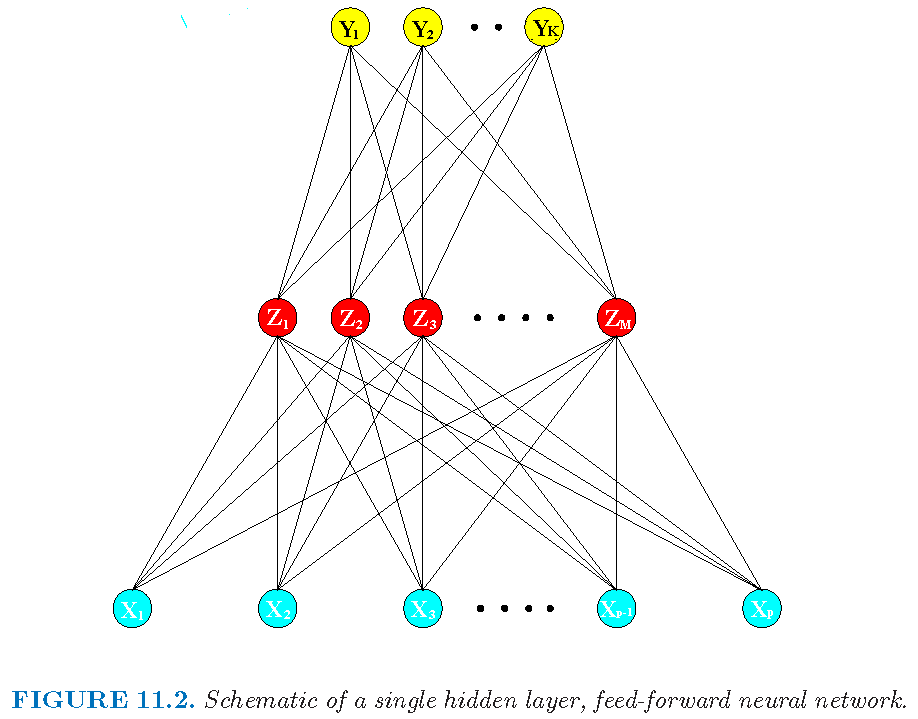
A feedforward vanilla NN with one hidden layer:
A vanilla neural network
Structure of a vanilla feedforward NN with one hidden layer:
- input layer to accept raw features
- hidden layer to transform features
- output layer to provide outputs
Derived features
Derived features \(Z_{m},m=1,\ldots,M\) are created from linear transforms of feature vector \(X\):
Linearly transformed features: \[\tilde{x}_m=\alpha_{0m}+\alpha_{m}^{T}X,m=1,\ldots,M\] for some parameters \(\alpha_{0m} \in \mathbb{R}\) and \(\alpha_{m} \in \mathbb{R}^p\) and \(M\)
- Derived features: \[ Z_{m} =\sigma\left( \tilde{x}_m \right), m=1,\ldots,M \] for a prespecified scalar function \(\sigma\), called activation function
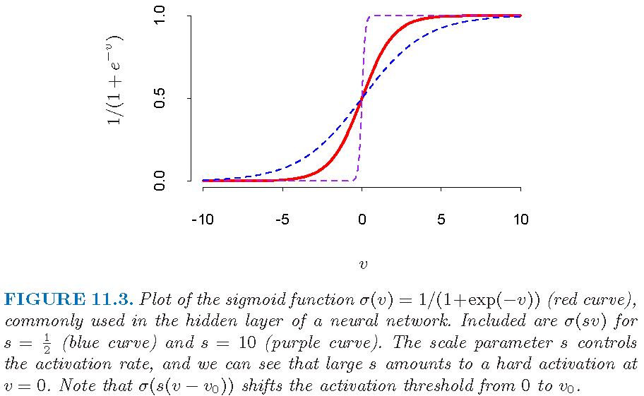
\(\sigma\) is often a sigmoid function as \[\sigma(v)=1/(1+e^{-v}), v \in \mathbb{R}\]
A sigmoid function
A sigmoid (i.e., S-shaped) function with two asymptotes:
Derived features and hidden layer
- Linearly transformed features \[\tilde{x}_m=\alpha_{0m}+\alpha_{m}^{T}X,m=1,\ldots,M\] attempt to “capture” or “extract” some properties of the \(p\) features \(X=(X_1,\ldots,X_p)^T\)
- From original feature vector \(X \in \mathbb{R}^p\) to derived feature vector \(Z=(Z_1,\ldots,Z_M)^T \in \mathbb{R}^M\), we see that the value of \(M\) indicates a “reduction” of feature space if \(M < p\) or an “extension” of feature space if \(M >p\), in terms of the number of “input features” to be processed by follow-up layers
- Units in NN that obtain derived features form a hidden layer since these features are not directly observable
Terminal mappings
- Linear transform on derived features: \[ T_{k} =\beta_{0k}+\beta_{k}^{T}Z,k=1,\dots,K \] for parameters \(\beta_{0k} \in \mathbb{R}\) and \(\beta_k \in \mathbb{R}^M\), where \(Z=(Z_1,\ldots,Z_M)^T \in \mathbb{R}^M\) is the vector of derived features
- Outputs: set \[ f_{k}\left( X\right)= g_{k}\left( T\right), k=1,\ldots,K \] where \(X\) is the feature vector, \(T=\left(T_{1},...,T_{K}\right)^T \in \mathbb{R}^{K}\), and each \(g_k: \mathbb{R}^K \to \mathbb{R}\) is some prespecified function. Here \(f_k: \mathbb{R}^p \to \mathbb{R}\) is defined via \(g_k\)
Note: the dimension of \(T\) is equal to \(K\), the number of classes
Summary on vanilla NN
A vanilla NN is a nonlinear mapping \(f: \mathbb{R}^p \to \mathbb{R}^K\) whose \(k\)th component mapping is \[ \begin{aligned} & f_k(X) = g_k(T) = g_k(\beta_{01}+\beta_{1}^{T}Z,\ldots,\beta_{0K}+\beta_{K}^{T}Z)\\ & = g_k\left(\beta_{01}+\beta_{1}^{T} (\sigma\left( \alpha_{01}+\alpha_{1}^{T}X \right),\ldots,\sigma\left( \alpha_{0M}+\alpha_{M}^{T}X \right))^T,\ldots, \right. \\ & \phantom{{}=1} \left. \beta_{0K}+\beta_{K}^{T} (\sigma\left( \alpha_{01}+\alpha_{1}^{T}X \right),\ldots,\sigma\left( \alpha_{0M}+\alpha_{M}^{T}X \right))^T \right) \end{aligned} \]
The more layes an NN has and more nonlinear functions an NN uses, the more complicated the mapping from the input vector \(X\) to output vector \(Y=(Y_1,\ldots,Y_k)^T\) is, and the harder it is to analyze the NN
Choice of terminal mappings
- For a regression task, \(g_{k}\) is usually set to be the \(k\)th coordinate function, i.e., \[g_{k}\left( T\right) =T_{k} \quad \text{ where } \quad T=(T_1,\ldots,T_K)^T\]
- For a classification task, \(g_{k}\) is set to be the softmax function as \[g_{k}\left( T\right) = \frac{e^{T_{k}}}{\sum_{l=1}^{K}e^{T_{l}}} \] Note that \(g_k\) is the transform used in the multi-class logistic (i.e., multilogit) classification task
Decision rule for classification
- Recall the \(k\)th component mapping: \[f_k(X)=g_k(T) = \frac{e^{T_{k}}}{\sum_{l=1}^{K}e^{T_{l}}}\]
- Classification rule: let \[\hat{k}=\operatorname{argmax}_{1 \le k \le K}g_k(T)\] Then \(X\) is classified into Class \(\hat{k}\), i.e., \(Y_{\hat{k}}=1\) but all other \(Y_{k}=0, k\ne \hat{k}\) are set
Note: the above decision rule is similar to the Bayes decision rule
Architecture of vanilla NN
A feedforward vanilla NN with one hidden layer:
Architecture of vanilla NN
The feedforward vanilla NN we have discussed has:
Activation function \(\sigma\), often as the sigmoid function \[\sigma\left(v\right)=1/\left(1+e^{-v}\right)\]
Terminal mappings \(g_k\), often as the softmax function \[g_{k}\left( T\right) = \frac{e^{T_{k}}}{\sum_{l=1}^{K}e^{T_{l}}} \] for a \(K\)-class classification task
Architectrue: forward and 3 layers (1 input layer, 1 hidden layer, and 1 output layer)
Architecture of neural networks
In general, the architecture of an NN
- can be single-layer or multi-layer
- can be feedforward only or feedforward with feedback loops
- can employ different transforms for different neurons or layers
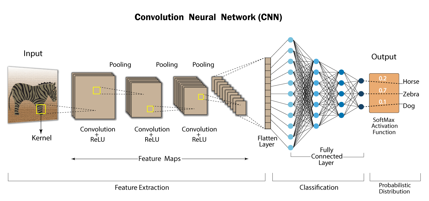
Convolutional neural networks (CNNs) are powerful models for image analysis, natural language processing, drug discovery, Go game, etc, and they employ convolution operations and the rectifier as activation function
Convolutional neural network
Forward; multilayer; with convolution operators; with rectifier as activation function:
Convolutional neural network
Looped; multilayer; with convolution operators; with rectifier as activation function:
Top 10 CNN architectures
Top 10 CNNs for classification:
 Credit: towardsdatascience.com
Estimating NN parameters
Unknown parameters of an NN are called “weights” and are stored in a vector \(\theta\)
We seek values of \(\theta\) that make the model fit the data well based on a criterion
For the vanilla NN, \(\theta\) consists of \(M\left(p+1\right)\) weights \[ \alpha_{0m} \in \mathbb{R},\alpha_{m} \in \mathbb{R}^p, m=1,\ldots,M \] and \(K\left( M+1\right)\) weights \[ \beta_{0k} \in \mathbb{R},\beta_{k}\in \mathbb{R}^M, k=1,\ldots,K \]
Note: activation function \(\sigma\) and terminal functions \(g_k\) are prespecified and do not need to be estimated
Objective functions
Given \(n\) observations \(\left\{ x_{i}\right\} _{i=1}^{n}\) for \(X\) and \(n\) observations \(\left\{ y_{ik}\right\} _{i=1}^{n}\) for each \(Y_{k},k=1,\ldots,K\):
- For regression, a criterion is the sum of squared errors \[ R\left( \theta\right) =\sum_{k=1}^{K}\sum_{i=1}^{n}\left( y_{ik} -f_{k}\left( x_{i}\right) \right)^{2} \]
- For classification, a criterion is the cross-entropy \[ R\left( \theta\right) =-\sum_{k=1}^{K}\sum_{i=1}^{n}y_{ik}\log f_{k}\left( x_{i}\right), \] and the corresponding classifier is \[\hat{Y}\left( x\right)=\operatorname{argmax}_{1 \le k \le K}f_{k}\left( x\right), x\in\mathbb{R}^{p}\]
Optimization and issues
Number of hidden units and layers relates to number of weights and level of complexity of an NN
Minimizing either criterion, usually done via gradient descent and if a minimizer \(\hat{\theta}\) exists, gives a choice of \(\theta\)
However, an NN is often over-parametrized, and we do not seek for a global minimizer \(\hat{\theta}\) of \(R\left( \theta\right)\) to potentially avoid overfitting. So, regularization on weights \(\theta\) is recommended to mitigate overfitting, and/or a validation dataset is used to check for overfitting
Optimization and issues
When optimizing \(R\left( \theta\right)\), starting values for weights are chosen to be random values near zero
Multiple minima: \(R\left( \theta\right)\) is often nonconvex and possesses many local minima. So, a minimizer \(\hat{\theta}\) may heavily depend on the initial values for the weights. One recommendation is to try a number of random starting configurations for the NN
There are many things we do not understand about NNs
Neural networks: software implementation
R software and commands
- R package
neuralnetthat builds simple neural networks - For a classification task, the commands
neuralnet,computeandplotfrom packageneuralnet
Command neuralnet
neuralnet{neuralnet} trains neural networks. It allows flexible settings through custom-choice of error and activation function. Its basic syntax is:
neuralnet(formula, data, hidden = 1,err.fct = "sse",
act.fct = "logistic", linear.output = TRUE,...)formula: a symbolic description of the model to be fitteddata: a data frame containing the variables specified informulahidden: a vector of integers specifying the number of hidden neurons in each hidden layer, and the length of the vector is the number of hidden layers
Command neuralnet
Basic syntax:
neuralnet(formula, data, hidden = 1,err.fct = "sse",
act.fct = "logistic", linear.output = FALSE,...)err.fct: a differentiable function that is used for the calculation of the error. Alternatively, the strings “sse” (for the sum of squared errors) and “ce” (for the cross-entropy) can be used
Command neuralnet
Basic syntax:
neuralnet(formula, data, hidden = 1,err.fct = "sse",
act.fct = "logistic", linear.output = FALSE,...)act.fct: a differentiable function that is used to obtain derived features, i.e., activation function. Additionally the strings, “logistic” and “tanh” are possible for the logistic function and tangent hyperbolicus, respectively. Alogisticactivation function is a sigmoid functionlinear.output: logical. Ifact.fctshould not be applied to the output neurons, setlinear.outputto beTRUE; otherwise, set it to beFALSE
Command neuralnet
neuralnet returns an object of class nn that is a list containing the following components:
model.list: a list containing the covariates and the response variables extracted from theformulaargumenterr.fctandact.fct: the error function and activation function, respectivelynet.result: a list containing the overall result of the neural network for every repetition
Command neuralnet
neuralnet returns an object of class nn that is a list containing the following components:
weights: a list containing the fitted weights of the neural network for every repetitionresult.matrix: a matrix containing the reached threshold, needed steps, error, AIC and BIC (if computed) and weights for every repetition. Each column represents one repetitionstartweights: a list containing the start weights of the neural network for every repetition
Command compute
compute{neuralnet} provides prediction of neural network of class nn, produced by neuralnet(). Its basic syntax is:
neuralnet::compute(x, covariate,rep = 1)x: an object of classnncovariate: a data frame or matrix containing the variables that had been used to train the neural networkrep: an integer indicating the neural network’s repetition which should be used
Command compute
compute{neuralnet} returns a list containing the following components:
neurons: a list of the neurons’ output for each layer of the neural networknet.result: a matrix withnrow(covariate)rows andKcolumns, whereKis the number of classes. Thek-th column contains the predicted probability that an observation belongs to classk
Note: compute{neuralnet} is replaced by predict.nn{neuralnet}, and the latter only returns the equivalent of net.result
Obtain class labels
Codes to obtain estimated class labels:
nnpred = neuralnet::compute(x, covariate,rep = 1)
classProbs = nnpred$net.result
if (which.max(classProbs[i,])==k) LabelEst[i]=k- assign observation \(x_i\) to class
kif the probability of \(x_i\) belonging to classkis the largest, i.e., \[k =\operatorname{argmax}_{1 \le j \le K} g_j(T),\] where \[f_j(X) = g_j(T) = \frac{e^{T_{j}}}{\sum_{l=1}^{K}e^{T_{l}}},\] \(X\) is the feature vector, \(f_j\) the \(j\)-th component mapping in the NN, and \(T=(T_1,\ldots,T_K)^T\)
Streamlined commands
Streamlined commands to obtain estimated class labels from an NN:
# fit model
nnfit=neuralnet(formula, data, hidden = 1,err.fct = "sse",
          act.fct = "logistic", linear.output = FALSE,...)
# obtain predicted class probabilities
nnpred=neuralnet::compute(nnfit,covariate)
classProbs = nnpred$net.result
# assign class labels
LabelEst = rep(1,nrow(covariate))
for (i in 1:nrow(covariate)) {
 if (which.max(classProbs[i,])==k)  LabelEst[i]=k
}
Command predict.nn
predict.nn{neuralnet} provides prediction of neural network of class nn, produced by neuralnet(). Its basic syntax is:
predict(object, newdata, rep = 1, all.units = FALSE, ...)object: neural network of classnnnewdata: new data of classdata.frameormatrixrep: integer indicating the neural network’s repetition which should be usedall.units: return output for all units instead of final output only...: further arguments passed to or from other methods
Command predict.nn
predict.nn{neuralnet} returns a matrix of predictions:
- each column of the matrix represents one output unit. If
all.units=TRUE, a list of matrices with output for each unit will be given - the matrix is equivalent to component
net.resultreturned bycompute{neuralnet}
Command plot.nn
plot.nn{neuralnet} is a method for the generic plot. It is designed for an inspection of the weights for objects of class nn, typically produced by neuralnet. Its basic syntax is:
plot(x,rep="best",intercept=F,information=F,
show.weights=F,col.hidden="blue")x: an object of classnnrep: repetition of the neural network. Ifrep="best", the repetition with the smallest error will be plotted. If not stated, all repetitions will be plotted, each in a separate window
Command plot.nn
Basic syntax:
plot(x,rep="best",intercept=F,information=F,
show.weights=F,col.hidden="blue")intercept: a logical value indicating whether to plot the interceptinformation: a logical value indicating whether to add the error and steps to the plotcol.hidden: color of the neurons in the hidden layer(s)
Neural networks: Example 1
On codes for example
Codes for example are adopted from
Iris flower data
- For each of 3 species “setosa”, “versicolor”, “virginica” of irises, 50 observations on 4 features
Sepal.Length,Sepal.Width,Petal.LengthandPetal.Widthare stored in objectiris(in R libraryggplot2orclass)
> library(class); dim(iris)
[1] 150   5
> iris[1,]
  Sepal.Length Sepal.Width Petal.Length Petal.Width Species
1          5.1         3.5          1.4         0.2  setosa
> unique(iris$Species)
[1] setosa     versicolor virginica
Levels: setosa versicolor virginica- The target is to classify an iris plant into one of the three species using these features
Data splitting and cross-validation
Proposal for data splitting and cross-validation (cv):
- 80% of data as training set that contains 40 random samples for each species, and the rest 20% as test set
- apply “\(5\)-fold cross-validation” on the training set to choose an optimal NN
Then apply optimal NN to test set
> library(class); set.seed(314) # seed needed!!
> trainId=c(sample(1:50,40),sample(51:100,40),
+           sample(101:150,40))
> testId = (1:150)[-trainId]
> trainingSet=iris[trainId,]; testSet=iris[testId,1:4]
> testLabs=iris$Species[testId]
> trainingLabs=iris$Species[trainId]
> m=5
> folds=sample(1:m,nrow(trainingSet),replace=TRUE)
Architecture of NN
- Input layer accepting 4 features, i.e., 4 neurons in input layer
- Two hidden layers: 5 neurons for hidden layer 1, and 4 neurons for hidden layer 2
- Output layer giving 3 class probabilities, i.e., 3 neurons in output layer
Codes for the architecture:
neuralnet(Species~., data, hidden = c(5,4),
           act.fct = "logistic",linear.output = FALSE)
Architecture of NN
> nnTrain=neuralnet(Species~., trainingSet, hidden = c(5,4),
+          act.fct = "logistic",linear.output = FALSE)
> library(neuralnet)
> plot(nnTrain,show.weights=F,information=F,intercept=F,
+      rep="best",col.hidden="blue")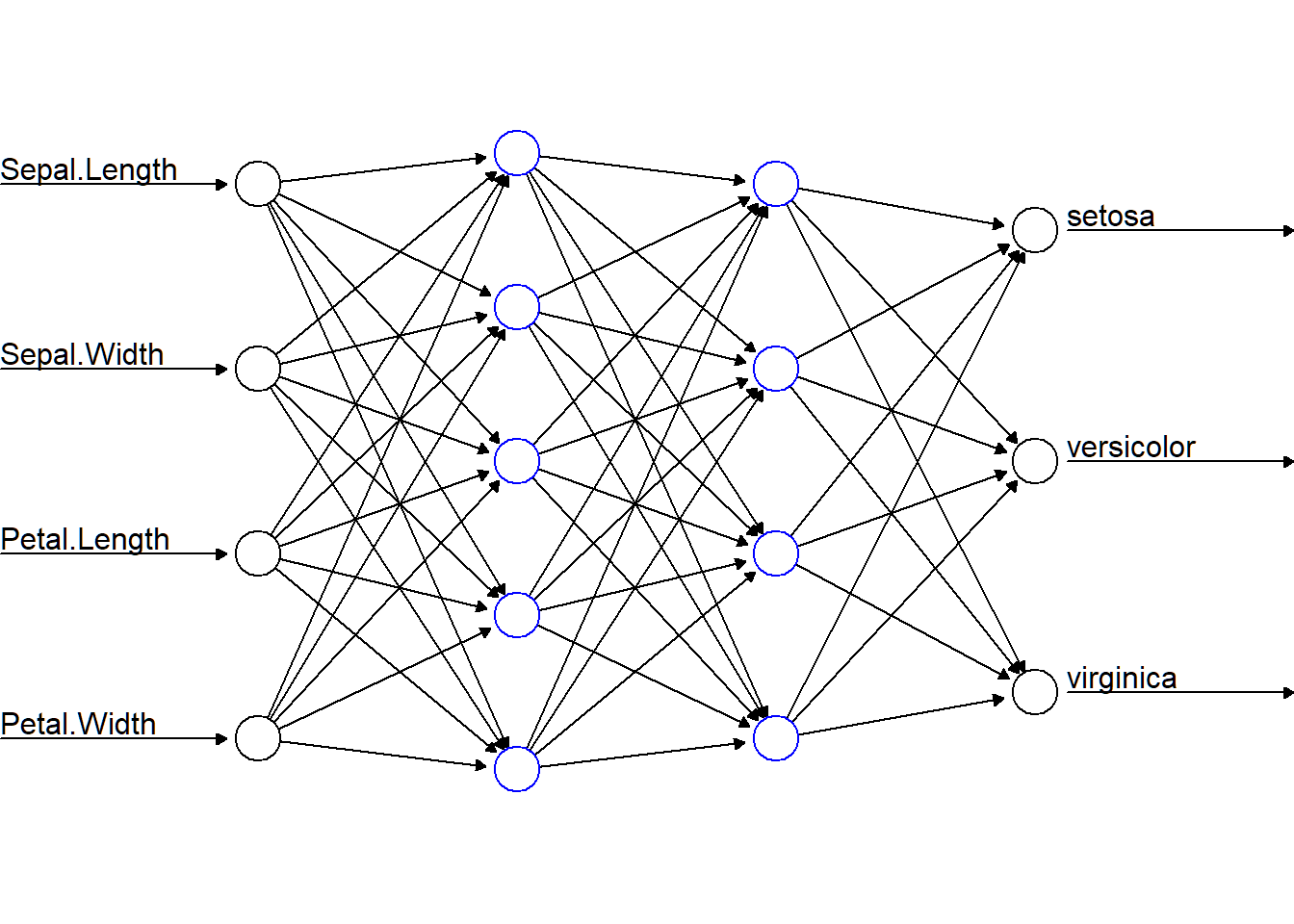
Cross-validation
\(5\)-fold cv for NN classifier on training Set:
> library(neuralnet); set.seed(123)
> nnModels = vector("list",m) # save each estimated model
> testErrorCV = double(m)
> for (s in 1:m) {
+   trainingTmp =trainingSet[folds !=s,]
+   testTmp =trainingSet[folds==s,]
+   testLabsTmp =trainingLabs[folds==s]
+   # fit the NN model
+   nnetTmp=neuralnet(Species~., trainingTmp, hidden = c(5,4),
+                  act.fct = "logistic",linear.output = FALSE)
+   nnModels[[s]]=nnetTmp
+   ypred = neuralnet::compute(nnetTmp, testTmp)
+   yhat = ypred$net.result
+   # assign labels
+   SpeciesEst=data.frame(
+     "labelEst"=ifelse(max.col(yhat[ ,1:3])==1,"setosa",
+       ifelse(max.col(yhat[ ,1:3])==2,
+              "versicolor", "virginica")))
+   SpeciesEst=factor(SpeciesEst[,1])
+   nOfMissObs= sum(1-as.numeric(testLabsTmp==SpeciesEst))
+   terror=nOfMissObs/length(testLabsTmp) # test error
+   testErrorCV[s]=terror
+ } # end of loop- models saved in
nnModels
Optimal NN model
Cross-validated test error:
> testErrorCV
[1] 0.05263158 0.00000000 0.03448276 0.08000000 0.00000000
>  mean(testErrorCV)
[1] 0.03342287
>  sd(testErrorCV)
[1] 0.034546
Optimal NN model:
> optNNnumber=min(which(testErrorCV==min(testErrorCV)))
> optNNnumber
[1] 2
> # extract and save optimal NN model
> optNNModel=nnModels[[optNNnumber]]
Apply optimal NN model
Apply optimal NN model to test set:
> NNOptPred=neuralnet::compute(nnModels[[optNNnumber]],testSet)
> yhatOPt= NNOptPred$net.result
> SpeciesEstOpt=data.frame(
+   "labelEst"=ifelse(max.col(yhatOPt[ ,1:3])==1,"setosa",
+       ifelse(max.col(yhatOPt[ ,1:3])==2,
+              "versicolor", "virginica")))
> SpeciesEstOpt=factor(SpeciesEstOpt[,1])
> nOfMissObsOPt= sum(1-as.numeric(testLabs==SpeciesEstOpt))
> terrorOPt=nOfMissObsOPt/length(testLabs) # test error
> table(SpeciesEstOpt,testLabs)
             testLabs
SpeciesEstOpt setosa versicolor virginica
   setosa         10          0         0
   versicolor      0          9         0
virginica 0 1 10- only 1 observation misclassified; error rate \(1/30\)
Visualization via 2 features
> testSet$Species=testLabs; testSet$EstSpecies=SpeciesEstOpt
> library(ggplot2); ggplot(testSet,aes(Sepal.Width,Petal.Length))+
+   geom_point(aes(shape=EstSpecies,color=Species))+theme_bw()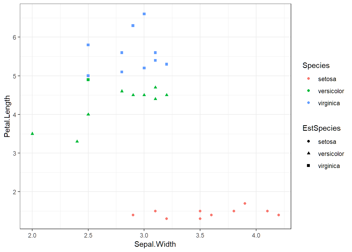
License and session Information
> sessionInfo()
R version 3.5.0 (2018-04-23)
Platform: x86_64-w64-mingw32/x64 (64-bit)
Running under: Windows 10 x64 (build 19041)

Matrix products: default

locale:
[1] LC_COLLATE=English_United States.1252
[2] LC_CTYPE=English_United States.1252
[3] LC_MONETARY=English_United States.1252
[4] LC_NUMERIC=C
[5] LC_TIME=English_United States.1252

attached base packages:
[1] stats     graphics  grDevices utils     datasets  methods
[7] base

other attached packages:
[1] knitr_1.21

loaded via a namespace (and not attached):
 [1] compiler_3.5.0  magrittr_1.5    tools_3.5.0
 [4] htmltools_0.3.6 revealjs_0.9    yaml_2.2.0
 [7] Rcpp_1.0.0      stringi_1.2.4   rmarkdown_1.11
[10] stringr_1.3.1   xfun_0.4        digest_0.6.18
[13] evaluate_0.12