Overview

Dimension reduction

• utilizes a low-dimensional structure, if existent, in data
• provides simple representation and visualization of data
• employs some mapping, and implicitly or explicitly optimizes some criterion

Dimension reduction techniques can be roughly categorized into:

• linear dimension reduction methods
• nonlinear dimension reduction methods

Learning submoduels

We will cover

• some key concepts in linear algebra
• principal components, curves and surfaces
• multidimensional scaling
• software implementation

Contents

The contents are adapted or adopted from:

• mainly Chapter 10 of the Text “An Introduction to Statistical Learning with Applications in R (Corrected at 8th printing)”
• partially Chapter 14 of the Supplementary Text “The Elements of Statistical Learning: Data Mining, Inference, and Prediction (2nd Edition)”
• other sources

Linear space

• A linear space \(\mathcal{V}\) over the set \(\mathbb{R}\) of real numbers is a set \(\mathcal{V}\) of “vectors” such that \[a\mathbf{v}+b\mathbf{w} \in \mathcal{V}\] for all \(\mathbf{v}, \mathbf{w} \in \mathcal{V}\) and \(a,b \in \mathbb{R}\)

• \(r\) vectors \(\mathbf{v}_1,\ldots,\mathbf{v}_r \in \mathcal{V}\) are linearly independent if and only if the linear combination \[a_1 \mathbf{v}_1 + \ldots + a_r \mathbf{v}_r=0\] for some \(a_1,\ldots,a_r \in \mathbb{R}\) implies that \(a_i=0\) for all \(i=1,\ldots,r\)

Linear space

• A linear space \(\mathcal{V}\) is said to have dimension \(s >0\), denoted by \(\text{dim}(\mathcal{V})=s\), if and only if there exit \(s\) linearly independent vectors \(\mathbf{w}_1,\ldots, \mathbf{w}_s \in \mathcal{V}\) such that any vector \(\mathbf{w}\) in \(\mathcal{V}\) can be written as a linear combination of these \(s\) vectors, i.e., any \[\mathbf{w}=b_1 \mathbf{v}_1 + \ldots + b_s \mathbf{v}_s\] for some \(b_1,\ldots,b_s \in \mathbb{R}\). The \(s\) vectors \(\mathbf{v}_1,\ldots, \mathbf{v}_s\) is called a basis for \(\mathcal{V}\)

• If a linear space \(\mathcal{V}\) has dimension \(s\), then any set of \(s\) linearly independent vectors of \(\mathcal{V}\) is a basis for \(\mathcal{V}\)

Euclidean space

• The \(p\)-dimensional Euclidean space \(\mathbb{R}^p\) is a vector space with canonical basis \(\{\mathbf{e}_i\}_{i=1}^p\), where \(\mathbf{e}_i\) is the \(p\)-dimensional vector with all \(0\) entries except for the \(i\)-th entry
• For \(\mathbf{a}=(a_1,\ldots,a_p)^T, \mathbf{b}=(b_1,\ldots,b_p)^T \in \mathbb{R}^p\), their Euclidean inner product is \[\langle \mathbf{a}, \mathbf{b}\rangle = \sum\nolimits_{i=1}^p a_i b_i,\] and \(\mathbf{a}\) and \(\mathbf{b}\) are orthogonal to each other if \(\langle \mathbf{a}, \mathbf{b}\rangle=0\)
• The Euclidean length or norm of \(\mathbf{a}\) is \[\Vert \mathbf{a} \Vert = \sqrt{\langle \mathbf{a}, \mathbf{a}\rangle}= \left(\sum\nolimits_{i=1}^p a_i^2\right)^{1/2}\]
• \(\mathbf{a}\) is called a unit vector if \(\Vert \mathbf{a} \Vert=1\)

Euclidean space

• The basis \(\{\mathbf{e}_i\}_{i=1}^p\) for \(\mathbb{R}^p\) is an orthogonal basis of \(\mathbb{R}^p\) since \[\langle \mathbf{e}_i, \mathbf{e}_j\rangle=0, i \ne j\] and further is an orthonormal basis since \[\Vert \mathbf{e}_i\Vert=1, \forall i=1,\ldots,p\]

• There are many other (not necessarily orthogonal or orthonormal) bases for \(\mathbb{R}^p\)

• A Euclidean space has many interesting and agreeable properties and is where most statistical learning tasks happen

Linear span

• Given \(d\) vectors \(\mathbf{w}_1,\ldots, \mathbf{w}_d \in \mathcal{V}\), their linear span (or span for short), denoted by \(\text{span}\left(\{\mathbf{w}_i\}_{i=1}^d\right)\), is the linear subspace of \(\mathcal{V}\) that contains all linear combinations of these \(d\) vectors, i.e., \[ \begin{aligned} \text{span}\left(\{\mathbf{w}_i\}_{i=1}^d\right)= \{\mathbf{w} \in \mathcal{V}: \mathbf{w}=b_1 \mathbf{v}_1 + \ldots + b_s \mathbf{v}_s,\\ \exists b_1, \ldots,b_s \in \mathbb{R}\} \end{aligned} \]

• The linear subspace \(\text{span}\left(\{\mathbf{w}_i\}_{i=1}^d\right)\) has dimension \(d\) if and only if \(\{\mathbf{w}_i\}_{i=1}^d\) are linearly independent

• A vector space \(\mathcal{V}\) is always the linear span of any of its basis

Basis and linear span

Two bases \(\{\mathbf{e}_1,\mathbf{e}_2\}\) and \(\{\mathbf{b}_1,\mathbf{b}_2\}\) for \(\mathbb{R}^2\), and their linear spans are just \(\mathbb{R}^2\)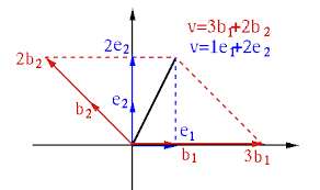

Linear span: examples

• For \(\mathbf{a} \in \mathbb{R}^p\), \(\text{span}\left(\mathbf{a}\right)\) is the line in \(\mathbb{R}^p\) that passes through \(\mathbf{a}\) and the origin \(0\)

• For linearly independent \(\mathbf{a}, \mathbf{b}\in \mathbb{R}^3\), \(\text{span}\left(\mathbf{a},\mathbf{b}\right)\) is the plane in \(\mathbb{R}^3\) that passes through \(\mathbf{a}\), \(\mathbf{b}\) and \(0\)

• For linearly dependent \(\mathbf{a}, \mathbf{b}\in \mathbb{R}^p\), \(\text{span}\left(\mathbf{a},\mathbf{b}\right)\) is the line in \(\mathbb{R}^p\) that passes through \(\mathbf{a}\), \(\mathbf{b}\) and \(0\)

Note: the concept of linear space will be used by the 2nd interpretation of principal component analysis, and the concept of orthogonality and basis will be used in the 1st interpretation of principal component analysis

Matrix as mapping

Consider an \(n \times p\) matrix \(\mathbf{A}=(a_{ij})\), a vector \(\mathbf{v} \in \mathbb{R}^p\) and a vector \(\mathbf{z} \in \mathbb{R}^n\). Then

• via right action \(\mathbf{A}\) maps \(\mathbf{z}\) to a vector in \(\mathbb{R}^p\), i.e., \[ \mathbf{A}: \mathbb{R}^n \to \mathbb{R}^p \quad \text{such that} \quad \mathbf{z} \mapsto \mathbf{z}^T\mathbf{A} \]

• via left action \(\mathbf{A}\) maps \(\mathbf{v}\) to a vector in \(\mathbb{R}^n\), i.e., \[ \mathbf{A}: \mathbb{R}^p \to \mathbb{R}^n \quad \text{such that} \quad \mathbf{v} \mapsto \mathbf{A}\mathbf{v} \]

• if \(p=n\), then either left or right action induces a mapping \(\mathbf{A}: \mathbb{R}^p \to \mathbb{R}^p\)

Eigenvalue and eigenvector

Consider a \(p \times p\) matrix \(\mathbf{A}\) and the mapping \(\mathbf{A}: \mathbb{R}^p \to \mathbb{R}^p\) via left action. If a nonzero vector \(\mathbf{v} \in \mathbb{R}^p\) is such that \[ \mathbf{A}\mathbf{v} = \lambda \mathbf{v} \] for some number \(\lambda\), then \(\lambda\) is called an eigenvalue of \(\mathbf{A}\), \(\mathbf{v}\) is an eigenvector associated with \(\lambda\), and \((\lambda,\mathbf{v})\) an eigenpair for \(\mathbf{A}\)

• If \(\mathbf{v}\) is an eigenvector associated with the eigenvalue \(\lambda\), then any \(a\mathbf{v}\) with \(a\ne 0\) is also an eigenvector associated with \(\lambda\). So, an eigenvector is often normalized to have Euclidean norm \(1\) and is then determined up to a \(\pm\) sign
• An eigenvalue can be the zero number but an eigenvector cannot be the zero vector

Geometric meaning of eigenpair

Let \((\lambda,\mathbf{v})\) be an eigenpair for the \(p\times p\) matrix \(\mathbf{A}\), i.e., \[\mathbf{A}\mathbf{v} = \lambda \mathbf{v}\]

• Then \[ \mathbf{A}(a\mathbf{v}) = a\mathbf{A}\mathbf{v}= (a\lambda) \mathbf{v}, \forall a \in \mathbb{R} \]
• However, the linear subspace spanned by \(\mathbf{v}\) is \[ \text{span}\left(\mathbf{v}\right)= \{\mathbf{w}\in \mathbb{R}^p: \mathbf{w}=a \mathbf{v},a \in \mathbb{R}\} \] So, for all \(\mathbf{w} \in \text{span}\left(\mathbf{v}\right)\), \[ \mathbf{A}\mathbf{w}=\mathbf{A}(a\mathbf{v}) = a\mathbf{A}\mathbf{v}= a\lambda \mathbf{v} \in \text{span}\left(\mathbf{v}\right), \] i.e., \(\mathbf{A}\) maps the linear subspace \(\text{span}\left(\mathbf{v}\right)\) into itself

Invariance: in summary, the linear subspace spanned by \(\mathbf{v}\) is invariant under the mapping \(\mathbf{A}\) if \(\mathbf{v}\) is an eigenvector of \(\mathbf{A}\)

Geometric meaning of eigenpair

Consider a \(p\times p\) matrix \(\mathbf{A}\), a vector \(\mathbf{v}\), and \(\tilde{\mathbf{v}}=\mathbf{A}\mathbf{v}\)

• The squared Euclidean norm of \(\tilde{\mathbf{v}}\) is \[ \begin{aligned} \Vert \tilde{\mathbf{v}} \Vert^2 =\langle\tilde{\mathbf{v}},\tilde{\mathbf{v}} \rangle=\tilde{\mathbf{v}}^T\tilde{\mathbf{v}} = (\mathbf{A}\mathbf{v})^T\mathbf{A}\mathbf{v} = \mathbf{v}^T (\mathbf{A}^T\mathbf{A})\mathbf{v} \end{aligned} \]
• If \((\lambda,\mathbf{v})\) is an eigenpair for \(\mathbf{A}\), then \(\mathbf{A}\mathbf{v} = \lambda \mathbf{v}\) and \[ \begin{aligned} \Vert \tilde{\mathbf{v}} \Vert^2 = (\mathbf{A}\mathbf{v})^T\mathbf{A}\mathbf{v}=\lambda \mathbf{v}^T \lambda \mathbf{v} = \lambda^2 \mathbf{v}^T\mathbf{v} = \lambda^2 \Vert \mathbf{v} \Vert^2 \end{aligned} \]

i.e., \[ \mathbf{A}\mathbf{v} = \lambda \mathbf{v} \implies \Vert \mathbf{A}\mathbf{v} \Vert = \vert\lambda\vert \Vert \mathbf{v} \Vert \]

Scaling: in summary, if \((\lambda,\mathbf{v})\) is an eigenpair for \(\mathbf{A}\), then the Euclidean norm (or length) of the image \(\mathbf{A}\mathbf{v}\) of \(\mathbf{v}\) is equal to \(\vert\lambda\vert\) times the Euclidean norm of \(\mathbf{v}\)

Orthogonal matrix and length

Consider a \(p\times p\) matrix \(\mathbf{A}\), a vector \(\mathbf{v}\), and \(\tilde{\mathbf{v}}=\mathbf{A}\mathbf{v}\)

• Recall the squared Euclidean norm of \(\tilde{\mathbf{v}}\) is \[ \begin{aligned} \Vert \tilde{\mathbf{v}} \Vert^2 =\langle\tilde{\mathbf{v}},\tilde{\mathbf{v}} \rangle=\tilde{\mathbf{v}}^T\tilde{\mathbf{v}} = (\mathbf{A}\mathbf{v})^T\mathbf{A}\mathbf{v} = \mathbf{v}^T (\mathbf{A}^T\mathbf{A})\mathbf{v} \end{aligned} \]

• If \(\mathbf{A}\) is an orthogonal matrix, i.e., \[\mathbf{A}\mathbf{A}^T=\mathbf{A}^T\mathbf{A}=\mathbf{I}_p,\] where \(\mathbf{I}_s\) is the identity matrix of dimension \(s\), then \[ \Vert \tilde{\mathbf{v}} \Vert^2 = \mathbf{v}^T (\mathbf{A}^T\mathbf{A})\mathbf{v} = \mathbf{v}^T \mathbf{I}_p\mathbf{v} = \Vert \mathbf{v} \Vert^2 \]

Length invariance: in summary, the Euclidean norm (or length) of the image \(\mathbf{A}\mathbf{v}\) of \(\mathbf{v}\) is equal to the Euclidean norm of \(\mathbf{v}\) if \(\mathbf{A}\) is an orthogonal matrix

Orthogonal matrix and basis

Let \(\mathbf{A}\) be a \(p\times p\) orthogonal matrix, i.e., \(\mathbf{A}\mathbf{A}^T=\mathbf{I}_p\), and let \(\{\mathbf{a}_i\}_{i=1}^p\) be the rows of \(\mathbf{A}\), and \(\{\mathbf{b}_i\}_{i=1}^p\) the columns of \(\mathbf{A}\)

• Orthogonality for rows and for columns (in Euclidean inner product): \[\langle \mathbf{a}_i, \mathbf{a}_j\rangle = \langle \mathbf{b}_i, \mathbf{b}_j\rangle=0, i \ne j\]
• Normalization (in Euclidean length): \[\Vert \mathbf{a}_i\Vert= \Vert \mathbf{b}_i\Vert=1, \forall i=1,\ldots,p\]
• Transpose is inverse: \(\mathbf{A}^{-1} = \mathbf{A}^T\)
• Transpose \(\mathbf{A}^T\) is also an orthogonal matrix

Orthonormal basis: the rows or columns of a \(p\times p\) orthogonal matrix form an orthonormal basis for \(\mathbb{R}^p\)

Singular value decompsosition

For an \(n \times p\) matrix \(\mathbf{A}\), consider the mapping \[ \mathbf{A}: \mathbb{R}^p \to \mathbb{R}^n \quad \text{such that} \quad \mathbf{v} \mapsto \mathbf{A}\mathbf{v} \] via left action

• Then there are an orthonormal basis \(\{\mathbf{u}_i\}_{i=1}^n\) for \(\mathbb{R}^n\) and an orthonormal basis \(\{\mathbf{v}_i\}_{i=1}^p\) for \(\mathbb{R}^p\), such that \[ \left\{ \begin{array} {ll} \mathbf{A}\mathbf{v}_i= d_i\mathbf{u}_i & \forall i=1,\ldots,\min\{n,p\} \\ \mathbf{A}\mathbf{v}_i=0 & \forall i> \min\{n,p\} \end{array}\right. \]

• The above representation is called the singular value decompsosition (SVD) of \(\mathbf{A}\). Each \(\mathbf{u}_i\) and \(\mathbf{v}_i\) is called a left and right singular vector, respectively, associated with singular value \(d_i\)

Singular value decompsosition

• Let \(\mathbf{V}=(\mathbf{v}_1,\ldots,\mathbf{v}_p)\), \(\mathbf{U}=(\mathbf{u}_1,\ldots,\mathbf{u}_n)\) and \[ \mathbf{D}=\left( \begin{array} [c]{cccc} d_{1} & 0 & \cdots & 0\\ 0 & \ddots & 0 & \vdots\\ \vdots & & d_{\min\{n,p\}} & 0\\ 0 & \cdots & 0 & 0 \end{array} \right) \in \mathbb{R}^{n \times p} \] Then \(\mathbf{U} \mathbf{U}^T= \mathbf{I}_n\) and \(\mathbf{V} \mathbf{V}^T= \mathbf{I}_p\)

• SVD for \(\mathbf{A}\) in matrix form is \[ \mathbf{A} = \mathbf{U} \mathbf{D} \mathbf{V}^T \]

Note: SVD is very fundamental!

Spectral decomposition

For a \(p \times p\) symmetric matrix \(\mathbf{A}=(a_{ij})\), i.e., \(\mathbf{A}^T=\mathbf{A}\), we have the spectral decomposition theorem:

• There exit an orthogonal matrix \(\mathbf{V}\) and a diagonal matrix \(\mathbf{D}\) such that \[ \mathbf{A}\mathbf{v}_i = d_i \mathbf{v}_i \iff \mathbf{A}\mathbf{V} = \mathbf{V} \mathbf{D} \iff \mathbf{A} = \mathbf{V} \mathbf{D} \mathbf{V}^T, \] where \(\mathbf{v}_i\) is the \(i\)-th column of \(\mathbf{V}\) and \(d_i\) the \(i\)-th diagonal entry of \(\mathbf{D}\) and each \((d_i,\mathbf{v}_i)\) is an eigenpair
• Further, \(\sum_{i=1}^p a_{ii}=\sum_{i=1}^p d_i\)

Namely, there exist an orthonormal basis \(\{\mathbf{v}_i\}_{i=1}^p\) for \(\mathbb{R}^p\) and scalars \(\{d_i\}_{i=1}^p\) such that \(\mathbf{A}\mathbf{v}_i = d_i \mathbf{v}_i\)

Note: spectral decomposition is very fundamental!

Positive semi-definiteness

• A \(p \times p\) symmetric matrix \(\mathbf{A}\) is said to be positive semi-defininte and denoted by \(\mathbf{A} \succeq 0\) if \[ \mathbf{v}^T \mathbf{A} \mathbf{v} \ge 0, \quad \forall \text{ nonzero } \mathbf{v} \in \mathbb{R}^p \] If \(\mathbf{v}^T \mathbf{A} \mathbf{v} > 0,\forall \text{ nonzero } \mathbf{v} \in \mathbb{R}^p\), then \(\mathbf{A}\) is said to be positive definite and denoted by \(\mathbf{A} \succ 0\)

• For \(r\) stochastically linearly independent random variables \(X_1,\ldots,X_s\), i.e., \[ a_1 X_1 + \ldots + a_s X_s=0 \implies a_1=\ldots=a_s=0 \] with probability \(1\), their covariance matrix \(\Sigma \succ 0\); otherwise, \(\Sigma \succeq 0\)

Positive semi-definiteness

Spectral decomposition for a \(p \times p\) symmetric matrix \(\mathbf{A}\) as \[ \mathbf{A}\mathbf{v}_i = d_i \mathbf{v}_i \iff \mathbf{A} = \mathbf{V} \mathbf{D} \mathbf{V}^T \] for an orthogonal matrix \(\mathbf{V}=(\mathbf{v}_1,\ldots,\mathbf{v}_p)\) and a diagonal matrix \(\mathbf{D}=\text{diag}\{d_1,\ldots,d_p\}\) implies:

• All eigenvalues \(d_i\) of \(\mathbf{A}\) are positive iff \(\mathbf{A}\) is positive definite, i.e., \(\mathbf{A} \succ 0 \iff \min_{1 \le i \le p}d_i >0\)
• All eigenvalues \(d_i\) of \(\mathbf{A}\) are non-negative iff \(\mathbf{A}\) is positive semi-definite, i.e., \(\mathbf{A} \succeq 0 \iff \min_{1 \le i \le p}d_i \ge 0\)
• For any \(n \times p\) matrix \(\mathbf{A}\), \(\mathbf{A}\mathbf{A}^T \succeq 0\) and \(\mathbf{A}^T\mathbf{A} \succeq 0\) (seen from SVD)

Note: positive semi-definiteness is very fundamental

Image under symmetric matrix

Consider a \(p \times p\) symmetric matrix \(\mathbf{A}\), a vector \(\mathbf{v} \in \mathbb{R}^p\), and its image \(\tilde{\mathbf{v}}=\mathbf{A}\mathbf{v} \in \mathbb{R}^p\)

• Spectral decomposition says there are an orthogonal matrix \(\mathbf{V}\) and a diagonal matrix \(\mathbf{D}\) such that \[ \mathbf{A} = \mathbf{V} \mathbf{D} \mathbf{V}^T \]
• Since an orthogonal matrix \(\mathbf{V}\) is equivalent to a rotation and a diagonal matrix to scaling, the image \[\tilde{\mathbf{v}}=\mathbf{A}\mathbf{v}=\mathbf{V} \mathbf{D} \mathbf{V}^T \mathbf{v}\] and is obtained by rotation (by \(\mathbf{V}^T\)), scaling (by \(\mathbf{D}\)) and rotation (by \(\mathbf{V}\)) of \(\mathbf{v}\) successively

Summary: a symmetric matrix as a mapping has a very intuitive geometric interpretation

Maximal scaled length

Consider an \(n \times p\) matrix \(\mathbf{A}\), a vector \(\mathbf{v} \in \mathbb{R}^p\), and its image \(\tilde{\mathbf{v}}=\mathbf{A}\mathbf{v} \in \mathbb{R}^n\)

• Recall the squared Euclidean norm of \(\tilde{\mathbf{v}}\) is \[ \begin{aligned} \Vert \tilde{\mathbf{v}} \Vert^2 =\langle\tilde{\mathbf{v}},\tilde{\mathbf{v}} \rangle=\tilde{\mathbf{v}}^T\tilde{\mathbf{v}} = (\mathbf{A}\mathbf{v})^T\mathbf{A}\mathbf{v} = \mathbf{v}^T (\mathbf{A}^T\mathbf{A})\mathbf{v} \end{aligned} \]
• Spectral decomposition of \[ \mathbf{B}=\mathbf{A}^T\mathbf{A}=\mathbf{V} \mathbf{D} \mathbf{V}^T \in \mathbb{R}^{p \times p}; \quad \mathbf{B}\succeq 0 \] with \(\mathbf{V}^T\mathbf{V}=\mathbf{I}_p\) and \(\mathbf{D}=\text{diag}\{d_1,\ldots,d_p\}\) implies \[ \begin{aligned} \mathbf{v}^T (\mathbf{A}^T\mathbf{A})\mathbf{v} = \mathbf{v}^T (\mathbf{V} \mathbf{D} \mathbf{V}^T)\mathbf{v} = (\mathbf{V}^T\mathbf{v})^T \mathbf{D} (\mathbf{V}^T\mathbf{v}) \end{aligned} \]
• Let \(\mathbf{a}=\mathbf{V}^T\mathbf{v}=(a_1,\ldots,a_p)^T\) and \(d_0=\max_{1 \le i \le n} d_i\). Then \(\Vert\mathbf{a}\Vert= \sqrt{\sum\nolimits_{i=1}^p a_i^2}=\Vert \mathbf{v}\Vert\) and \[ \Vert \tilde{\mathbf{v}} \Vert^2=\mathbf{a}^T \mathbf{D} \mathbf{a} \le d_0 \sum\nolimits_{i=1}^p a_i^2 = d_0 \Vert \mathbf{v}\Vert^2 \]

Maximal scaled length

• Recap as the maximal scaled length lemma: Let \(\mathbf{A} \in \mathbb{R}^{n \times p}\), \(\mathbf{v} \in \mathbb{R}^p\) and \(\tilde{\mathbf{v}}=\mathbf{A}\mathbf{v} \in \mathbb{R}^n\) and set \(d_0\) be the maximal eigenvalue of \(\mathbf{B}=\mathbf{A}^T\mathbf{A} \succeq 0\). Then \[ \Vert \tilde{\mathbf{v}} \Vert^2=\Vert \mathbf{A}\mathbf{v} \Vert^2 = \mathbf{v}^T \mathbf{B}\mathbf{v} \le d_0 \Vert \mathbf{v}\Vert^2 \] and \[ \Vert \tilde{\mathbf{v}} \Vert=\Vert \mathbf{A}\mathbf{v} \Vert = \sqrt{ \mathbf{v}^T \mathbf{B}\mathbf{v}} \le \sqrt{d_0} \Vert \mathbf{v}\Vert \] Here \(d_0\) is called the spectral norm of \(\mathbf{B}\) when \(\mathbf{B} \succeq 0\)
• If further \(\Vert \mathbf{v} \Vert=1\), then \[ \Vert \mathbf{A} \mathbf{v} \Vert^2= \mathbf{v}^T \mathbf{B}\mathbf{v} \le d_0 \]
• Summary: the maximum of \(\Vert\mathbf{A}\mathbf{v}\Vert^2\), i.e., the maximum of the “scaled” length \(\mathbf{v}^T \mathbf{B}\mathbf{v}\), subject to \(\Vert \mathbf{v} \Vert=1\), cannot exceed the spectral norm of \(\mathbf{B}\) (when \(\mathbf{B} \succeq 0\))

Maximal scaled length

For \(\mathbf{B} \in \mathbb{R}^{p \times p}\) and \(\mathbf{B} \succeq 0\),

• Spectral decomposition: \(\mathbf{B}=\mathbf{V} \mathbf{D} \mathbf{V}^T\) with \(\mathbf{V}^T\mathbf{V}=\mathbf{I}_p\) and \(\mathbf{D}=\text{diag}\{d_1,\ldots,d_p\}\) and \(\mathbf{V}=(\mathbf{v}_1,\ldots,\mathbf{v}_p)\)
• Arrange columns of \(\mathbf{V}\) so that \((d_i,\mathbf{v}_i)\) is an eigenpair and \[d_1=\max\nolimits_{1 \le i \le p} d_i=d_0\]
• Then maximal scaled length lemma implies that \[ \mathbf{v}^T \mathbf{B}\mathbf{v} \le d_0=d_1=d_1 \Vert \mathbf{v}_1\Vert^2=\mathbf{v}_1^T \mathbf{B}\mathbf{v}_1 \] for \(\Vert \mathbf{v}\Vert=1\). Namely, \[ \mathbf{v}_1=\operatorname{argmax}_{\Vert \mathbf{v}\Vert=1} \mathbf{v}^T \mathbf{B}\mathbf{v}; \quad \max\nolimits_{\Vert \mathbf{v}\Vert=1}\mathbf{v}^T \mathbf{B}\mathbf{v}=d_1 \]

Note: Write \(d_1=\Vert \mathbf{B}\Vert_{\text{op}}\). Then \(\Vert \mathbf{B}\Vert_{\text{op}}\) for \(\mathbf{B} \succeq 0\) is the maximal scaling of the length of a unit vector

Trace and Frobenius norm

• For a \(p \times p\) matrix \(\mathbf{A}=(a_{ij})\), its trace is defined as \[ \text{tr}(\mathbf{A})= \sum\nolimits_{i=1}^p a_{ii} \] Namely, trace is the sum of diagonal entries

• For an \(n \times p\) matrix \(\mathbf{A}=(a_{ij})\), its Frobenius norm is defined as \[ \Vert \mathbf{A} \Vert_F = \sqrt{\sum\nolimits_{i=1}^n \sum\nolimits_{j=1}^p a_{ij}^2}=\sqrt{\text{tr}\left(\mathbf{A}^T \mathbf{A}\right)}=\sqrt{\text{tr}\left(\mathbf{A} \mathbf{A}^T\right)} \] Namely, the Frobenius norm of \(\mathbf{A}\) is the Euclidean norm of the vector obtained by stacking rows or columns of \(\mathbf{A}\)

Note: trace is a very fundamental

Summary

• Spectral decomposition and maximal scaled length are the methodology and theory behind both the population version and data version of principal data analysis (PCA)

• Singular value decomposition and maximal scaled length are the methodology and theory behind PCA as the best linear approximate to a data matrix under the Frobenius norm among all subspaces of dimensions upper bounded by a positive number

• Without sufficient understanding of the key concepts in linear algebra that have been discussed, one may have considerable difficulty well understanding, applying and interpreting PCA

Probabilistic formulation

• \(p\) stochastically linearly independent feature variables \(X_1,\ldots,X_p\) and feature vector \(X=(X_1,\ldots,X_p)^T\), i.e.,\[a_1 X_1 + \ldots + a_p X_p=0\] for some \(a_1,\ldots,a_p \in \mathbb{R}\) implies that \(a_i=0\) for all \(i=1,\ldots,p\) with probability \(1\)
• Each \(X_i\) has mean zero, i.e., \(\mathbb{E}(X_i)=0\), and finite variance \(\text{Var}(X_i)=\sigma_i^2\); so, \(\mathbb{E}(X)=0\)
• Covariance matrix of \(X\) is \(\Sigma\), and \(\Sigma \succ 0\), i.e., \(\Sigma\) is positive definite (since feature variables are stochastically linearly independent)

Note: \(\mathbb{E}\) denotes “expectation” and \(\text{Var}\) “variance”

Projecting feature vector

For \(p\) unit vectors \(\mathbf{v}_i=(\phi_{i1},\ldots,\phi_{ip})^T \in \mathbb{R}^p\) (i.e., \(\Vert \mathbf{v}_i\Vert=1\)), define linear combinations of \(X_j\)’s as \[ Z_i = \underbrace{\mathbf{v}_i^T X=\langle \mathbf{v}_i, X \rangle =\sum_{j=1}^p \phi_{ij}X_j}_{\text{definition of Euclidean inner product}}\in \mathbb{R} \]

• Then \(\mathbb{E}(Z_i)=\mathbb{E}(\sum_{j=1}^p \phi_{ij}X_j)=\sum_{j=1}^p \phi_{ij}\mathbb{E}(X_j)=0\) since \(\mathbb{E}(X_j)=0\)

Note: since \(\Vert \mathbf{v}_i\Vert=1\), we see \(Z_i=\langle \mathbf{v}_i, X \rangle\) is the projection of \(X\) onto \(\mathbf{v}_i\)

Variance of projection

• Since \(Z_i =\mathbf{v}_i^T X \in \mathbb{R}\) and \(\mathbb{E}(Z_i)=0\), we see \[ \begin{aligned} \delta_i&=\text{Var}(Z_i)=\underbrace{\text{Var}(\mathbf{v}_i^T X) =\mathbb{E}\left[(\mathbf{v}_i^T X)^2\right]=\mathbb{E}(\mathbf{v}_i^T X X^T \mathbf{v}_i)}_{\text{definition of variance}}\\ & \underbrace{=\mathbf{v}_i^T\mathbb{E}(XX^T)\mathbf{v}_i= \mathbf{v}_i^T \text{Cov}(X) \mathbf{v}_i}_{\text{definition of expectation}}=\mathbf{v}_i^T \Sigma \mathbf{v}_i \end{aligned} \]
• In summary, \[\delta_i=\text{Var}(Z_i)=\text{Var}(\mathbf{v}_i^T X)=\mathbf{v}_i^T \Sigma \mathbf{v}_i\]
• Namely, the variance \(\delta_i\) of \(Z_i\) is the squared Euclidean norm of \(\mathbf{v}_i\) “scaled” by \(\Sigma\)

Note: \(\text{Cov}\) denotes “covariance”

Covariances among projections

• Since \(Z_i =\mathbf{v}_i^T X \in \mathbb{R}\) and \(\mathbb{E}(Z_i)=0\), we see \[ \begin{aligned} \delta_{ij}&=\underbrace{\text{Cov}(Z_i,Z_j)=\mathbb{E}\left(\mathbf{v}_i^T X\mathbf{v}_j^T X\right)=\mathbb{E}(\mathbf{v}_i^T X X^T \mathbf{v}_j)}_{\text{definition of covariance}}\\ & \underbrace{=\mathbf{v}_i^T\mathbb{E}(XX^T)\mathbf{v}_j= \mathbf{v}_i^T \text{Cov}(X) \mathbf{v}_j}_{\text{definition of expectation}}=\mathbf{v}_i^T \Sigma \mathbf{v}_j \end{aligned} \]
• In summary, \[\delta_{ij}=\text{Cov}(Z_i,Z_j)=\mathbf{v}_i^T \Sigma \mathbf{v}_j.\]
• Namely, the covariance between \(Z_i\) and \(Z_j\) is the Euclidean inner product between \(\mathbf{v}_i\) and \(\mathbf{v}_j\) “scaled” by \(\Sigma\)

Recap on projections

• Feature vector \(X=(X_1,\ldots,X_p)^T\) with \(\mathbb{E}(X)=0\) and positive definite covariance matrix \(\Sigma \succ 0\)

• Projections \[ Z_i =\mathbf{v}_i^T X \in \mathbb{R} \quad \text{with} \quad \Vert \mathbf{v}_i\Vert=1, \] such that \[ \left\{ \begin{array} {ll} \mathbb{E}(Z_i)=0, & \forall i=1,\ldots,p \\ \delta_i=\text{Var}(Z_i)=\mathbf{v}_i^T \Sigma \mathbf{v}_i, &\forall i=1,\ldots,p\\ \delta_{ij}=\text{Cov}(Z_i,Z_j)=\mathbf{v}_i^T \Sigma \mathbf{v}_j, & \forall i\ne j \end{array}\right. \]

PCA: optimization

PCA aims to find \(p\) unit vectors \(\tilde{\mathbf{v}}_i \in \mathbb{R}^p,i=1,\ldots,p\) such that the projections \[ \tilde{Z}_i =\tilde{\mathbf{v}}_i^T X \in \mathbb{R} \quad \text{with} \quad \Vert \tilde{\mathbf{v}}_i\Vert=1, \] achieve

• mutual uncorrelateness: \[ \text{Cov}(\tilde{Z}_i,\tilde{Z}_j) =0 ,\forall i \ne j \]
• successive maximal variances: \[ \begin{aligned} \text{Var}(\tilde{Z}_1) \ge \text{Var}(\tilde{Z}_2) \ge \cdots \ge \text{Var}(\tilde{Z}_p);\\ \text{Var}(\tilde{Z}_i)=\max \left\{\text{Var}({Z}_i): {Z}_i={\mathbf{v}}_i^T X, \Vert {\mathbf{v}}_i\Vert=1,\right.\\ \quad \quad \quad \left. \langle \mathbf{v}_i,\mathbf{v}_j\rangle=0, i \ne j \right\} \end{aligned} \]
• total variance: \(\sum_{i=1}^p \text{Var}(\tilde{Z}_i)=\sum_{i=1}^p \text{Var}(X_i)\)

PCA: solution

• Let \(\Sigma\) have spectral decomposition as \[ \Sigma \tilde{\mathbf{v}}_i = d_i \tilde{\mathbf{v}}_i \iff \Sigma = \mathbf{V} \mathbf{D} \mathbf{V}^T \] for an orthogonal matrix \(\mathbf{V}=(\tilde{\mathbf{v}}_1,\ldots,\tilde{\mathbf{v}}_p)\) and a diagonal matrix \(\mathbf{D}=\text{diag}\{d_1,\ldots,d_p\}\)

• Then \(d_i>0,\forall i\) (since \(\Sigma \succ 0\)). Arrange columns of \(\mathbf{V}\) so that \[d_1 \ge d_2 \ge \ldots \ge d_p\]

• Since \(\delta_i=\text{Var}(Z_i)=\mathbf{v}_i^T \Sigma \mathbf{v}_i\), the maximal scaled length lemma implies that \[ \begin{aligned} d_i =\text{Var}(\tilde{\mathbf{v}}_i^T X)=\max \left\{\text{Var}({Z}_i): {Z}_i={\mathbf{v}}_i^T X, \Vert {\mathbf{v}}_i\Vert=1,\right.\\ \quad \quad \quad \left. \langle \mathbf{v}_i,\mathbf{v}_j\rangle=0, i \ne j \right\} \end{aligned} \]

PCA: solution

• Namely, successive maximal variances is achieved by setting \[ \tilde{Z}_i=\tilde{\mathbf{v}}_i^T X \] whose variance is the \(i\)-th largest eigenvalue \(d_i\) of \(\Sigma\), where \(\tilde{\mathbf{v}}_i\) is a unit eigenvector associated with \(d_i\)

• Since \(\tilde{\mathbf{v}}_i^T \tilde{\mathbf{v}}_j=0\) for \(i\ne j\), the covariance \[ \text{Cov}(\tilde{Z}_i,\tilde{Z}_j)=\tilde{\mathbf{v}}_i^T \Sigma \tilde{\mathbf{v}}_j=\tilde{\mathbf{v}}_i^T d_j \tilde{\mathbf{v}}_j=0. \] Namely, \(\tilde{Z}_i\)’s are mutually uncorrelated

• Each such \(\tilde{Z}_i\) is called a principal component, and \(\tilde{\mathbf{v}}_i\) the loading vector for \(\tilde{Z}_i\)

PCA: dimension reduction

• If we want to use no more than \(q < p\) projections \[ Z_i =\mathbf{v}_i^T X \in \mathbb{R} \text{ where } \Vert \mathbf{v}_i\Vert=1,\langle {\mathbf{v}}_i, \mathbf{v}_j \rangle=0,i\ne j \] that together explain an amount of variance for the feature vector \(X=(X_1,\ldots,X_p)^T\) measured by \[ \rho_q= \sum\nolimits_{i=1}^q \text{Var}(Z_i) \]
• then PCA provides an optimal solution \(\tilde{Z}_i=\tilde{\mathbf{v}}_i^T X\) with \(\text{Var}(\tilde{Z}_i)=d_i\) and maximal total variance \[ \sum\nolimits_{i=1}^q \text{Var}(\tilde{Z}_i) = \max_{Z_i,i=1,\ldots,q}\rho_q, \] where \(d_1,\ldots,d_q\) are the \(q\) largest eigenvalues of the covariance matrix \(\Sigma\) for \(X\) and \((d_i,\tilde{\mathbf{v}}_i)\) is an eigenpair for \(\Sigma\)

PCA: procedure

Summary: PCA projects feature vector \(X\) successively onto unit eigenvectors of the covariance matrix \(\Sigma\) of \(X\) that are associated with decreasingly ordered eigenvalues of \(\Sigma\)

PCA Procedure (population version):

• Obtain spectral decomposition \(\Sigma = \mathbf{V} \mathbf{D} \mathbf{V}^T\) for an orthogonal matrix \(\mathbf{V}=({\mathbf{v}}_1,\ldots,{\mathbf{v}}_p)\) and a diagonal matrix \(\mathbf{D}=\text{diag}\{d_1,\ldots,d_p\}\) such that \((d_i,{\mathbf{v}}_i)\) is an eigenpair for \(\Sigma\) and that \(d_1 \ge d_2 \ge \ldots \ge d_p > 0\)

• Define optimal projections \(Z_i={\mathbf{v}}_i^T X, i=1,\ldots,p\)

Overview

“PCA for a data matrix (referred to as data version PCA)” applies to the data matrix a family of projections in an optimal way:

• Data version PCA employs SVD of the data matrix (or equivalently spectral decomposition of a symmetric matrix induced by the data matrix)
• The projections are induced by singular vectors in the SVD of the data matrix (or equivalently by the orthonormal eigenvectors of the induced symmetric matrix)
• Data version PCA does not employ a probabilistic model and has two equivalent formulations

Settings

• \(p\) stochastically linearly independent features \(X_1,\ldots,X_p\) and feature vector \(X=(X_1,\ldots,X_p)^T\)
• \(n\) linearly independent observations \(x_i \in \mathbb{R}^p\) on \(X\), and data matrix \(\mathbf{X}=(x_{ij}) \in \mathbb{R}^{n \times p}\) whose \(i\)-th row is \(x_i\) (i.e., each column of \(\mathbf{X}\) is a feature and each row of \(\mathbf{X}\) is an observation)
• Features are centered, i.e., \(\mathbf{X}\) is column-centered such that \(n^{-1}\sum_{i=1}^n x_{ij}=0\) for all \(1 \le j \le p\)
• Since \(\mathbf{X}\) is column-centered, the rank of \(\mathbf{X}\), denoted by \(\text{rank}(\mathbf{X})\), is \(\min\{n-1,p\}\); if \(\mathbf{X}\) is neither column-centered nor row-centered, then \(\text{rank}(\mathbf{X})=\min\{n,p\}\)

PCA: optimization

PCA aims to find \(q \le r=\text{rank}(\mathbf{X})\) projections \[ \tilde{\mathbf{z}}_i =\mathbf{X}\tilde{\mathbf{v}}_i \in \mathbb{R}^n \quad \text{with} \quad \tilde{\mathbf{v}}_i\in \mathbb{R}^p,\Vert \tilde{\mathbf{v}}_i\Vert=1 \] of \(\mathbf{X}=(x_{ij})\) to achieve

• mutual orthogonality: \[ \tilde{\mathbf{v}}_i^T \tilde{\mathbf{v}}_j=0 \quad \text{and} \quad \langle \tilde{\mathbf{z}}_i,\tilde{\mathbf{z}}_j \rangle =0 ,\forall i \ne j \]
• successive maximal lengths: \[ \left\{ \begin{array} {l} \Vert \tilde{\mathbf{z}}_1 \Vert \ge \Vert \tilde{\mathbf{z}}_2 \Vert \ge \cdots \ge \Vert \tilde{\mathbf{z}}_{r} \Vert\\ \Vert \tilde{\mathbf{z}}_i \Vert=\max \left\{\Vert {\mathbf{z}}_i \Vert: {\mathbf{z}}_i=\mathbf{X}{\mathbf{v}}_i,{\mathbf{v}}_i\in \mathbb{R}^p,\Vert {\mathbf{v}}_i\Vert=1,\right.\\ \quad \quad \quad \quad \quad \quad \left.\langle \mathbf{v}_i,\mathbf{v}_j\rangle=0, i \ne j\right\} \end{array}\right. \]

• total variability: \[ \text{tr}(\mathbf{X}^T\mathbf{X})=\sum\nolimits_{i=1}^n \sum\nolimits_{j=1}^p x_{ij}^2=\sum\nolimits_{i=1}^{r} \Vert \tilde{\mathbf{z}}_i \Vert^2 \]

PCA: solution

• Let \(\mathbf{S}=\mathbf{X}^{T}\mathbf{X} \in \mathbb{R}^{p \times p}\). Since \(\mathbf{X}\) is centered, \((p-1)^{-1}\mathbf{S}\) is the sample covariance matrix of feature vector \(X\) if \(X\) is regarded as a random vector
• Let \(\mathbf{S}\) have spectral decomposition as \[ \mathbf{S}\tilde{\mathbf{v}}_i = d_i \tilde{\mathbf{v}}_i \iff \mathbf{S} = \mathbf{V} \mathbf{D} \mathbf{V}^T \] for an orthogonal matrix \(\mathbf{V}=(\tilde{\mathbf{v}}_1,\ldots,\tilde{\mathbf{v}}_p) \in \mathbb{R}^{p\times p}\) and a diagonal matrix \(\mathbf{D}=\text{diag}\{d_1,\ldots,d_p\}\) such that \[ d_1 \ge \cdots \ge d_{r} > 0 \] and \[ d_{r+1} = \cdots = d_{p} = 0 \] since \(\mathbf{X}\) has rank \(r\)

Note: general facts are stated above

PCA: solution

Setting \(\tilde{\mathbf{z}}_i =\mathbf{X}\tilde{\mathbf{v}}_i\) for \(1 \le i \le r\) gives

• mutual orthogonality: \(\tilde{\mathbf{v}}_i^T\tilde{\mathbf{v}}_j=0, i \ne j\) and \[ \langle \tilde{\mathbf{z}}_i,\tilde{\mathbf{z}}_j\rangle=\tilde{\mathbf{v}}_i^T\mathbf{X}^T\mathbf{X}\tilde{\mathbf{v}}_j=d_j\tilde{\mathbf{v}}_i^T\tilde{\mathbf{v}}_j=0, i \ne j \]
• successive maximal lengths: since \[ d_i=\Vert \tilde{\mathbf{z}}_i \Vert^2= \tilde{\mathbf{v}}_i^T\mathbf{X}^T\mathbf{X}\tilde{\mathbf{v}}_i, \] the maximal scaled length lemma implies that \[ \Vert \tilde{\mathbf{z}}_i \Vert=\max \left\{\Vert {\mathbf{z}}_i \Vert: {\mathbf{z}}_i=\mathbf{X}{\mathbf{v}}_i,\Vert {\mathbf{v}}_i\Vert=1,\langle {\mathbf{v}}_i, \mathbf{v}_j \rangle=0,i\ne j\right\} \]
• total variability: \[\sum\nolimits_{i=1}^n \sum\nolimits_{j=1}^p x_{ij}^2=\sum\nolimits_{i=1}^{r} \Vert \tilde{\mathbf{z}}_i \Vert^2\]

Note: \(\Vert \tilde{\mathbf{z}}_i \Vert^2\) is the variability of \(\mathbf{X}\) explained by \(\tilde{\mathbf{z}}_i\)

PCA: dimension reduction

• If we want to use no more than \(q \le \text{rank}(\mathbf{X})\) projections \[ {\mathbf{z}}_i=\mathbf{X}{\mathbf{v}}_i \text{ where } {\mathbf{v}}_i\in \mathbb{R}^p,\Vert {\mathbf{v}}_i\Vert=1,\langle {\mathbf{v}}_i, \mathbf{v}_j \rangle=0,i\ne j \] that together explain an amount of variability in data \(\mathbf{X}\) measured by \[ \rho_q= \sum\nolimits_{i=1}^q \Vert {\mathbf{z}}_i \Vert^2 \]
• then PCA provides an optimal solution \(\tilde{\mathbf{z}}_i =\mathbf{X}\tilde{\mathbf{v}}_i\) with \(\Vert \tilde{\mathbf{z}}_i \Vert^2=d_i\) and maximal total variability \[ \sum\nolimits_{i=1}^q \Vert \tilde{\mathbf{z}}_i \Vert^2 = \max_{{\mathbf{z}}_i,i=1,\ldots,q}\rho_q, \] where \(d_1,\ldots,d_q\) are the \(q\) largest eigenvalues of \(\mathbf{X}^{T}\mathbf{X}\) and \((d_i,\tilde{\mathbf{v}}_i)\) is an eigenpair for \(\mathbf{X}^{T}\mathbf{X}\)

Remarks on projections

• The \(i\)-th optimal projection \(\tilde{\mathbf{z}}_i =\mathbf{X}\tilde{\mathbf{v}}_i \in \mathbb{R}^n\) where \[ \tilde{\mathbf{v}}_i \in \mathbb{R}^p, \Vert \tilde{\mathbf{v}}_i\Vert=1, \langle \tilde{\mathbf{v}}_i,\tilde{\mathbf{v}}_j \rangle=0,i \ne j \] is called the \(i\)-th principal component score vector, and its entries are called the \(i\)th principal component scores

• The \(k\)-th entry of \(\tilde{\mathbf{z}}_i\) is \[ \tilde{z}_{ki}=x_k \tilde{\mathbf{v}}_i = \langle x_k^T, \tilde{\mathbf{v}}_i\rangle, 1\le k \le n \] and is the projection of the \(k\)-th observation \(x_k\) (a row vector) onto \(\tilde{\mathbf{v}}_i\)

• The unit vector \(\tilde{\mathbf{v}}_i\) is called the loading vector or direction for the \(i\)-th principal component

PCA: procedure

• Given \(n \times p\) data matrix \(\mathbf{X} \in \mathbb{R}^{n \times p}\) with \(r=\text{rank}(\mathbf{X})\), whose \(i\)-th row is observation \(x_i\) on \(p\) features

• Let \(\mathbf{S}=\mathbf{X}^{T}\mathbf{X}\) have spectral decomposition as \[ \mathbf{S}\tilde{\mathbf{v}}_i = d_i \tilde{\mathbf{v}}_i \iff \mathbf{S} = \mathbf{V} \mathbf{D} \mathbf{V}^T \] for an orthogonal matrix \(\mathbf{V}=(\tilde{\mathbf{v}}_1,\ldots,\tilde{\mathbf{v}}_p) \in \mathbb{R}^{p \times p}\) and a diagonal matrix \(\mathbf{D}=\text{diag}\{d_1,\ldots,d_p\}\) such that \[ d_1 \ge \cdots \ge d_{r} >0 \] and \[ d_{r+1} = \cdots = d_{p} = 0 \]

• Set \(\tilde{\mathbf{z}}_i =\mathbf{X}\tilde{\mathbf{v}}_i\) for \(1 \le i \le r\)

PCA: summary

• Population version PCA: since \(\left\{\tilde{\mathbf{v}}_{j}\right\}_{j=1}^{p}\) is an orthonormal basis for \(\mathbb{R}^{p}\), each \(\left\vert \tilde{\mathbf{v}}_{j}^T X\right\vert\) is the “projected length” of feature vector \(X\) onto the direction \(\tilde{\mathbf{v}}_{j}\), and \(\text{Var}(\tilde{\mathbf{v}}_{j}^T X)\) is the variability of \(X\) along the direction \(\tilde{\mathbf{v}}_{j}\)
• Data version PCA: since \(\left\{\tilde{\mathbf{v}}_{j}\right\}_{j=1}^{p}\) is an orthonormal basis for \(\mathbb{R}^{p}\), each \(\left\Vert \mathbf{X}\tilde{\mathbf{v}}_{j}\right\Vert\) is the “projected length” of data matrix \(\mathbf{X}\) onto the direction \(\tilde{\mathbf{v}}_{j}\), and \(\left\Vert \mathbf{X}\tilde{\mathbf{v}}_{j}\right\Vert^2\) is the variability of \(\mathbf{X}\) along the direction \(\tilde{\mathbf{v}}_{j}\)
• So, PCA projects the data matrix or feature vector onto mutually orthogonal directions along which features have successively maximal variabilities

Remarks

The presentation of data and population versions of PCA here are conceptually the same as that in Section 10.2 of the Text, except the following:

• Here vector and matrix notations are used, and more statistical and geometrical interpretations of key steps for PCA are provided

• Here a systematic treatment of linear dimension reduction based on spectral decomposition is provided

• Here \(n^{-1}\) given in the optimization settings in Section 10.2 of the Text is omitted, which does not affect the optimal solutions at all

Overview

• PCA provides the best linear approximate to observations in a data matrix \(\mathbf{X}\) in Frobenius norm among all subspaces of dimensions less than or equal to a given number

• This interpretation of PCA can be extended to propose and conduct nonlinear dimension reduction if we do not restrict ourselves to use linear subspaces

Settings

• \(p\) stochastically linearly independent features \(X_1,\ldots,X_p\) and feature vector \(X=(X_1,\ldots,X_p)^T\)

• \(n\) linearly independent observations \(x_i \in \mathbb{R}^p\) on \(X\), and data matrix \(\mathbf{X}=(x_{ij}) \in \mathbb{R}^{n \times p}\) whose \(i\)-th row is \(x_i\) (i.e., each column of \(\mathbf{X}\) is a feature and each row of \(\mathbf{X}\) is an observation)

• Features are centered, i.e., \(\mathbf{X}\) is column-centered such that \(n^{-1}\sum_{i=1}^n x_{ij}=0\) for all \(1 \le j \le p\)

Fixed rank linear model

Consider the rank \(q\) linear model \[ f\left(\boldsymbol{\beta}\right) = \boldsymbol{\mu} +\mathbf{V}_{q} \boldsymbol{\beta} \] for representing \(\left\{ x_{i}\right\}_{i=1}^{n}\), where

• the \(p\times q\) matrix \(\mathbf{V}_{q}\) has \(q\) orthonormal columns, i.e., columns of \(\mathbf{V}_{q}\) are mutually orthogonal and have unit norm
• \(\boldsymbol{\mu} \in\mathbb{R}^{p}\) is a location vector
• \(\boldsymbol{\beta} \in\mathbb{R}^{q}\) contains parameters

We want to find \(\boldsymbol{\beta}_i \in\mathbb{R}^{q}\) such that \(f\left(\boldsymbol{\beta}_i\right)\) reconstructs \(x_{i}\) for each \(i=1,\ldots,n\) in some optimal sense

Least squares fit

• The least squares fit of the model leads to \[ \min_{\boldsymbol{\mu},\mathbf{V}_{q}, \boldsymbol{\beta}_i,i=1,\ldots,n}\sum_{i=1} ^{n}\left\Vert x_{i}^T-\boldsymbol{\mu}-\mathbf{V}_{q}\boldsymbol{\beta}_i\right\Vert^{2}, \] whose critical point satisfies \(\hat{\boldsymbol{\mu}}=\bar{x}^T=n^{-1}\sum_{i=1}^n x_i^T=0\) (since \(\mathbf{X}\) is centered) and \[ \hat{\boldsymbol{\beta}}_{i}=\mathbf{V}_{q}^{T}\left(x_{i}^T-\bar{x}^T\right)=\mathbf{V}_{q}^{T}x_{i}^T \]
• The objective function (by definition of Frobenius norm) becomes \[ g(\mathbf{V}_{q})=\sum_{i=1}^{n}\left\Vert x_{i}^T-\mathbf{V}_{q} \mathbf{V}_{q}^{T}x_{i}^T\right\Vert ^{2}=\left\Vert \mathbf{X}^{T}-\mathbf{V}_{q}\mathbf{V}_{q}^{T}\mathbf{X}^{T}\right\Vert _{F}^{2}, \] where \(\Vert \cdot \Vert_F\) is the Frobenius norm

SVD for data matrix

Data matrix \(\mathbf{X}=(x_{ij}) \in \mathbb{R}^{n \times p}\) has singular value decompsosition (SVD) by:

• an orthonormal basis \(\{\mathbf{u}_i\}_{i=1}^n\) for \(\mathbb{R}^n\) and an orthonormal basis \(\{\mathbf{v}_i\}_{i=1}^p\) for \(\mathbb{R}^p\), such that \[ \left\{ \begin{array} {ll} \mathbf{X}\mathbf{v}_i= d_i\mathbf{u}_i & \forall i=1,\ldots,\min\{n,p\} \\ \mathbf{X}\mathbf{v}_i=0 & \forall i> \min\{n,p\} \end{array}\right. \] and that \[ \vert d_1 \vert \ge \vert d_2 \vert \ge \cdots \ge \vert d_{\min\{n,p\}} \vert \ge 0 = \cdots = 0 \]
• Let \(\mathbf{V}=(\mathbf{v}_1,\ldots,\mathbf{v}_p)\), \(\mathbf{U}=(\mathbf{u}_1,\ldots,\mathbf{u}_n)\). Then \(\mathbf{U} \mathbf{U}^T= \mathbf{I}_n\) and \(\mathbf{V} \mathbf{V}^T= \mathbf{I}_p\). Namely, \(\mathbf{V}\) and \(\mathbf{U}\) are orthogonal matrices of dimension \(p\) and \(n\), respectively

SVD for data matrix

• Recall \(\mathbf{V}=(\mathbf{v}_1,\ldots,\mathbf{v}_p)\) and \(\mathbf{U}=(\mathbf{u}_1,\ldots,\mathbf{u}_n)\). Set \[ \mathbf{D}=\left( \begin{array} [c]{cccc} d_{1} & 0 & \cdots & 0\\ 0 & \ddots & 0 & \vdots\\ \vdots & & d_{\min\{n,p\}} & 0\\ 0 & \cdots & 0 & 0 \end{array} \right) \in \mathbb{R}^{n \times p} \]

• Then SVD for \(\mathbf{X}\) in matrix form is \[ \mathbf{X} = \mathbf{U} \mathbf{D} \mathbf{V}^T \]

SVD of data matrix

• Recall the SVD \(\mathbf{X}=\mathbf{UDV}^{T}\)

• The SVD of \(\mathbf{X}\) gives the spectral decomposition of \(\mathbf{X}^{T}\mathbf{X}\) as \[ \mathbf{X}^{T}\mathbf{X}=\mathbf{V}\mathbf{D}^T\mathbf{U}^{T}\mathbf{UDV}^{T}=\mathbf{V}\mathbf{D}^T\mathbf{D}\mathbf{V}^{T} \]

• So, each eigenvalue \(\lambda_{i}\) of \(\mathbf{X}^{T}\mathbf{X}\) satisfies \(\lambda_{i}=d_{i}^{2}\) and the eigenvector \(\mathbf{a}_{i}\) of \(\mathbf{X}^{T}\mathbf{X}\) can be identified with the right singular vector \(\mathbf{v}_{i}\)

Note: SVD and spectral decomposition are intrinsically related

Optimal solution

The SVD \(\mathbf{X} = \mathbf{U} \mathbf{D} \mathbf{V}^T\) with \(\mathbf{V}=(\mathbf{v}_1,\ldots,\mathbf{v}_p)\) and some involving algebraic arguments imply:

• the solution to \[ \min_{\mathbf{V}_{q}}\left\Vert \mathbf{X}^{T}-\mathbf{V}_{q}\mathbf{V} _{q}^{T}\mathbf{X}^{T}\right\Vert_{F}^{2} = \min_{\mathbf{V}_{q}}g(\mathbf{V}_{q}) \] is \[\mathbf{\hat{V}}_{q}=\left( \mathbf{v}_{1},...,\mathbf{v}_{q}\right)\] for which \(\mathbf{v}_{i}\) is the \(i\)th column of \(\mathbf{V}\) (and hence is an eigenvector associated with the \(i\)th largest eigenvalue \(\lambda_{i}=d_i^2\) of \(\mathbf{X}^{T}\mathbf{X}=\mathbf{V}\mathbf{D}^T\mathbf{D}\mathbf{V}^T\))

PCA: summary

• Let \(\left\langle \mathbf{V}_{q}\right\rangle\) be the linear space spanned by the (orthonormal) columns of \(\mathbf{V}_{q}\) (i.e., column space of \(\mathbf{V}_{q}\)). Then \(\text{dim}(\left\langle \mathbf{V}_{q}\right\rangle)=q\). Since \(\mathbf{V}_{q}\mathbf{V}_{q}^{T}\) is a projection matrix, \(\mathbf{V}_{q}\mathbf{V}_{q}^{T}\mathbf{X}^{T}\) projects each row \(x_{i}\) of \(\mathbf{X}\) onto \(\left\langle \mathbf{V}_{q}\right\rangle\)
• The Frobenius norm \[ \left\Vert \mathbf{X}^{T}-\mathbf{V}_{q}\mathbf{V}_{q}^{T}\mathbf{X} ^{T}\right\Vert _{F}^{2}=\left\Vert \left( \mathbf{I}-\mathbf{V} _{q}\mathbf{V}_{q}^{T}\right) \mathbf{X}^{T}\right\Vert _{F}^{2} \] is the sum of residual squared Euclidean lengths of projecting all \(\left\{x_{i}\right\}_{i=1}^{n}\) onto \(\left\langle \mathbf{V}_{q}\right\rangle\), i.e., this Frobenius norm is the residual sum of squares for the least squares fit of the rank \(q\) linear model
• PCA provides the best linear approximate to \(\mathbf{X}\) in Frobenius norm among all subspaces of dimensions \(q\leq p\)

PCA: procedure

Recall the SVD \(\mathbf{X}=\mathbf{U}\mathbf{D}\mathbf{V}^{T}\)

• The optimal subspace is the column space of \(\mathbf{\hat{V}}_{q}\), the \(p\times q\) matrix that contains the first \(q\) columns of \(\mathbf{V}\) (that are associated with the \(q\) largest eigenvalues of \(\mathbf{X}^T\mathbf{X}\))

• The optimal \(\hat{\boldsymbol{\beta}}_{i}=\mathbf{\hat{V}}_{q}^{T}x_{i}^T \in \mathbb{R}^q\)

• Each column of \(\mathbf{UD}\) is called a “principal component score vector” of \(\mathbf{X}\) since \(\mathbf{X}\mathbf{V}=\mathbf{U}\mathbf{D}\)

• The fitted rank \(q\) linear model is \[x_{i}^T\approx\bar{x}^T+\mathbf{\hat{V}}_{q}\mathbf{\hat{V}}_{q}^{T}\left( x_{i}^T-\bar{x}^T\right)\]

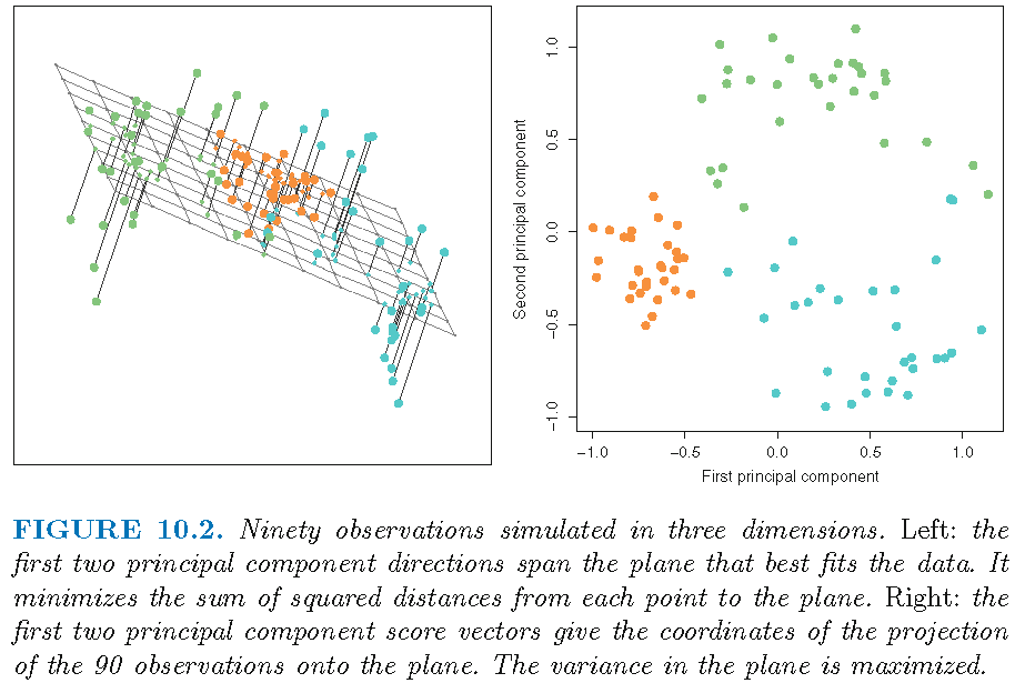
Illustration: optimal subspace

Directions are unit eigenvectors; scores are projections

License and session Information

License

> sessionInfo()
R version 3.5.0 (2018-04-23)
Platform: x86_64-w64-mingw32/x64 (64-bit)
Running under: Windows 10 x64 (build 19041)

Matrix products: default

locale:
[1] LC_COLLATE=English_United States.1252 
[2] LC_CTYPE=English_United States.1252   
[3] LC_MONETARY=English_United States.1252
[4] LC_NUMERIC=C                          
[5] LC_TIME=English_United States.1252    

attached base packages:
[1] stats     graphics  grDevices utils     datasets  methods  
[7] base     

other attached packages:
[1] knitr_1.21

loaded via a namespace (and not attached):
 [1] compiler_3.5.0  magrittr_1.5    tools_3.5.0    
 [4] htmltools_0.3.6 revealjs_0.9    yaml_2.2.0     
 [7] Rcpp_1.0.0      stringi_1.2.4   rmarkdown_1.11 
[10] stringr_1.3.1   xfun_0.4        digest_0.6.18  
[13] evaluate_0.12