Stat 437 Lecture Notes 8a
Xiongzhi Chen
Washington State University

Principal component analysis (PCA): Example 1
Data
The USArrests data set (included in the library ISLR or ggplot2) contains arrests per 100,000 residents in each of the 50 US states in 1973. There are
- 4 features: 3 types of crimes
Murder,Assault,Rape, andUrbanPop(percent of population living in urban areas)
> library(ISLR); dim(USArrests)
[1] 50  4
> head(USArrests)
           Murder Assault UrbanPop Rape
Alabama      13.2     236       58 21.2
Alaska       10.0     263       48 44.5
Arizona       8.1     294       80 31.0
Arkansas      8.8     190       50 19.5
California    9.0     276       91 40.6
Colorado      7.9     204       78 38.7
> colSums(USArrests)
  Murder  Assault UrbanPop     Rape
   389.4   8538.0   3277.0   1061.6
Initial assessment
Description of data:
- \(p=4\) (stochastically linearly independent) features \(X_1,\ldots,X_4\); otherwise, knowing any 3 features among the 4 features
Murder,Assault,RapeandUrbanPopenables us to know completely the remaining feature, and a 4th feature is redundant and does not have to be measured - \(n=50\) observations on feature vector \(X=(X_1,\ldots,X_4)^T\). These observations can be assumed to be linearly independent, since otherwise a linear combination of observations of features for some US states is equal to the observation for another US state and that observation is redundant
Initial assessment
Data matrix \(\mathbf{X} \in \mathbb{R}^{n \times p}\):
- These 50 observations are not necessarily stochastically independent since observations on the 4 features for states that have similar demographics, infrastructures and laws may be correlated
- So, it is sensible to assume that the data matrix \(\mathbf{X}\) has rank \(4=\min\{p,n\}\). However, \(\mathbf{X}\) is not column-centered
- We cannot implement population version PCA since we do not know the covariance matrix \(\Sigma\) of the feature vector \(X\)
- So, we will implement data version PCA to find optimal directions to project data matrix onto to capture maximal total variability in data successively
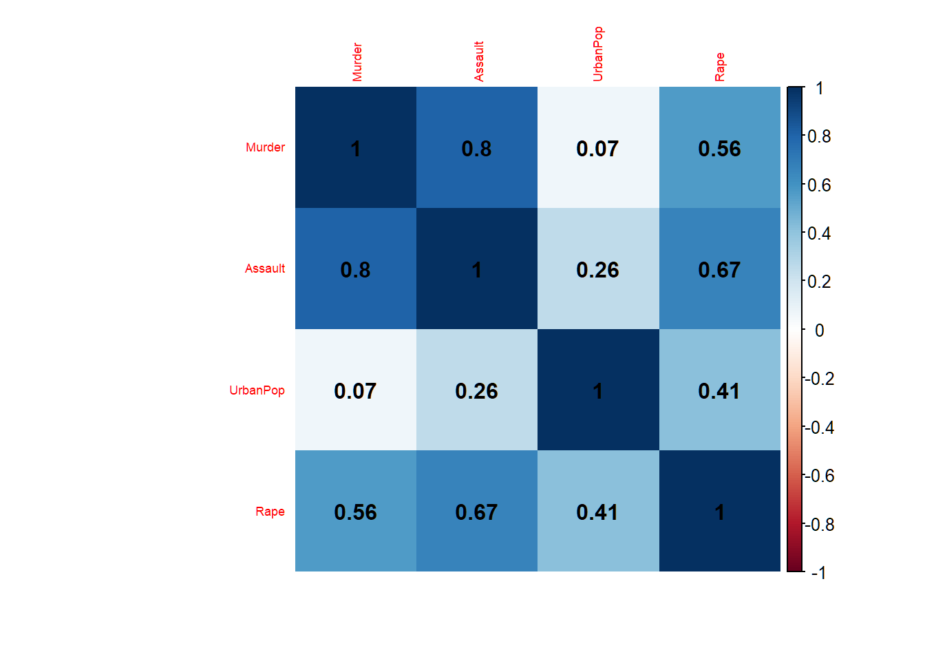
Correlations among features
4 features, each with 50 observations; Murder, Assault and Rape are considerably correlated; UrbanPop has low correlation with these 3 features
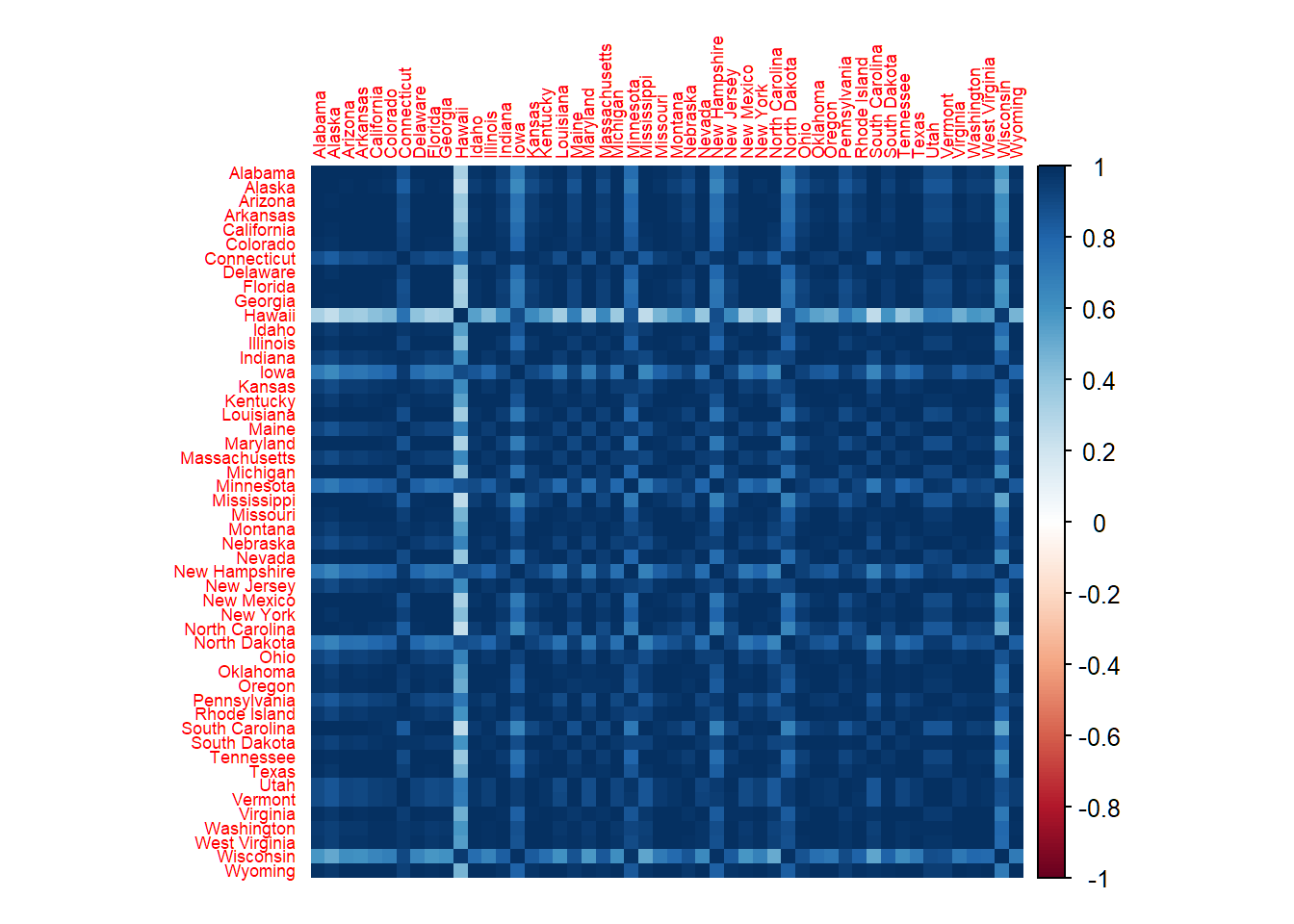
Correlations among observations
50 observations, each for a US state; sample correlation between two observations insensible for features
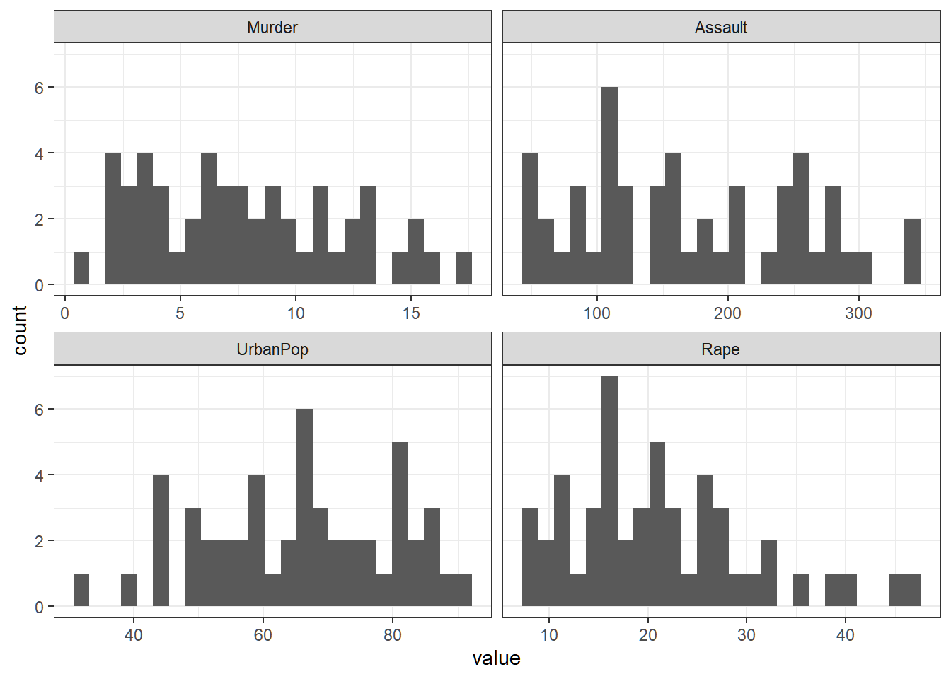
Variabilities of features
Variability of each (raw) feature
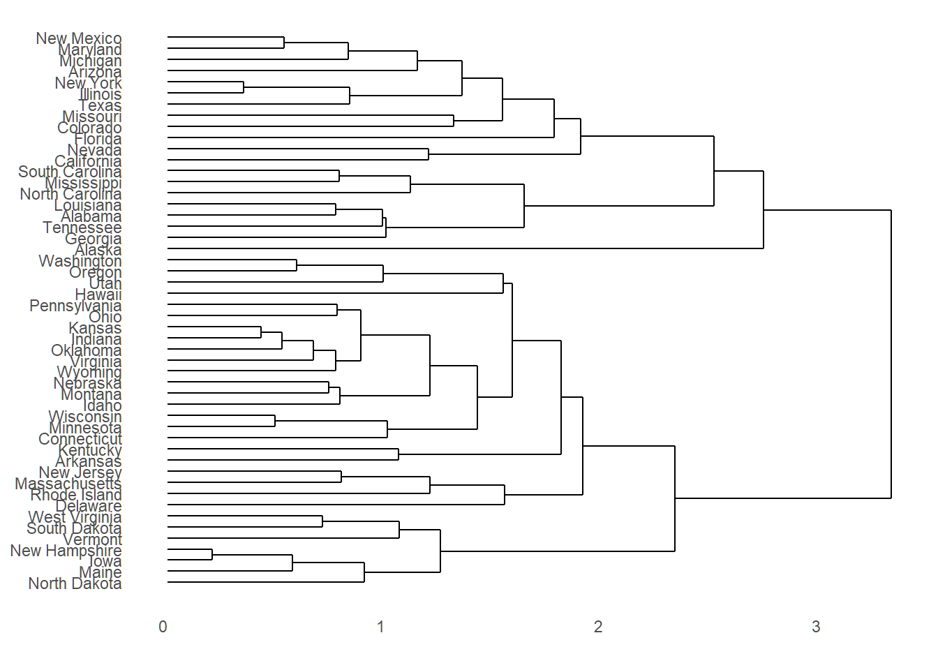
Dendrogram
Dendrogram does not reveal along which orthogonal directions observations vary the most successively
Standardizing data
- Settings: \(p=4\), \(n=50\), data matrix \(\mathbf{X}=(x_{ij}) \in \mathbb{R}^{n \times p}\) and \(\text{rank}(\mathbf{X})=4\)
- Center and scale data: let \[ \bar{x}_j=n^{-1}\sum_{i=1}^n x_{ij}; \quad s_j^2= \frac{1}{n-1}\sum_{i=1}^n (x_{ij}-\bar{x}_j)^2 \] and define “standardized data matrix” \(\tilde{\mathbf{X}}=(\tilde{x}_{ij})\) such that \[ \tilde{x}_{ij} = (x_{ij} - \bar{x}_j)/\sqrt{s_j^2} \]
- \(\bar{x}_j\) is the sample mean, and \(s_j^2\) and \(s_j\) are the sample variance and sample standard deviation of feature \(X_j\), respectively
Total variability
- Total variability of only centered data depends on magnitudes of measurements on features, i.e., for only column-centered \(\mathbf{X}=(x_{ij}) \in \mathbb{R}^{n \times p}\), \[ \text{tr}(\mathbf{X}^T\mathbf{X})=\sum_{i=1}^n \sum_{j=1}^p {x}_{ij}^2=(n-1)\sum_{j=1}^p s_j^2 \]
- Total variability of standardized data is completely determined by number of observations and number of features, i.e., for standardized data \(\tilde{\mathbf{X}}=(\tilde{x}_{ij}) \in \mathbb{R}^{n \times p}\), \[ \text{tr}(\tilde{\mathbf{X}}^T\tilde{\mathbf{X}})=\sum_{i=1}^n \sum_{j=1}^p \tilde{x}_{ij}^2 =(n-1)p \]
- It is recommended to standardize data before applying PCA
PCA of standardized data
- Let \(\{\tilde{\mathbf{v}}_i\}_{i=1}^p\) be the mutually orthogonal unit eigenvectors of \(\tilde{\mathbf{X}}^T\tilde{\mathbf{X}} \in \mathbb{R}^{p \times p}\) that are associated with descendingly ordered eigenvalues \(d_1 \ge \cdots \ge d_p>0\). Then the score vectors (i.e., projections) are \[ \tilde{\mathbf{z}}_i = \tilde{\mathbf{X}} \tilde{\mathbf{v}}_i \in \mathbb{R}^{n}, i=1,\ldots,p \]
- The \(r\)-th entry of \(\tilde{\mathbf{z}}_i\) is the projection of the \(r\)-th standardized observation \(\tilde{x}_r\) on \(X\) (and the \(r\)-th row of \(\tilde{\mathbf{X}}\)) onto \(\tilde{\mathbf{v}}_i\), i.e., \[ \tilde{z}_{ri}=\langle \tilde{x}_r^T, \tilde{\mathbf{v}}_i\rangle, r=1,\ldots,n \]
- \(\tilde{\mathbf{z}}_i\) is the score vector and \(\tilde{\mathbf{v}}_i\) the loading vector (i.e., direction of projection) respectively for the \(i\)-th principal component (PC). Entries of a \(\tilde{\mathbf{v}}_i\) are also called “weights”
A convention
For any positive semi-definite matrix \(\mathbf{A} \in \mathbb{R}^{p \times p}\) (whose eigenvalues are all non-negative) and any \(q \le \text{rank}(\mathbf{A})\), the orthonormal (i.e., mutually orthogonal, unit) eigenvectors (each determined up to \(\pm\) signs) that are associated with the \(q\) largest eigenvalues of \(\mathbf{A}\) are called “the first \(q\) eigenvectors” of \(\mathbf{A}\). The \(q\) largest eigenvalues of \(\mathbf{A}\) are called the first \(q\) eigenvalues of \(\mathbf{A}\)
Since each \((d_i,\tilde{\mathbf{v}}_i)\) is an eigenpair of \(\tilde{\mathbf{S}}=\tilde{\mathbf{X}}^T\tilde{\mathbf{X}}\) that has eigenvalues \(d_1 \ge \cdots \ge d_p>0\), then for any \(q \le p\), the orthonormal eigenvectors \(\{\tilde{\mathbf{v}}_i\}_{i=1}^q\) are the first \(q\) eigenvectors and \(d_1,\ldots,d_q\) the first \(q\) eigenvalues of \(\tilde{\mathbf{S}}\)
Dominant features
- Let the direction \(\tilde{\mathbf{v}}_i=(\phi_{i1},\ldots,\phi_{ip})^T\) for a fixed \(i\). If the \(s\)-th entry \(\phi_{is}\) of \(\tilde{\mathbf{v}}_i\) has absolute value that dominates those of other entries of \(\tilde{\mathbf{v}}_i\), then the projection of observation \(\tilde{x}_r\) onto \(\tilde{\mathbf{v}}_i\) \[ \tilde{z}_{ri}=\langle \tilde{x}_r^T, \tilde{\mathbf{v}}_i\rangle =\sum\nolimits_{j=1}^p \tilde{x}_{rj}\phi_{ij}\approx \tilde{x}_{rs}\phi_{is} \] and hence the projection of standardized data matrix \(\tilde{\mathbf{X}}\) onto \(\tilde{\mathbf{v}}_i\) \[ \tilde{\mathbf{z}}_i \approx \phi_{is} \tilde{\mathbf{x}}_s, \] where \(\tilde{\mathbf{x}}_s\) is the \(s\)-th column of \(\tilde{\mathbf{X}}\) that contains \(n\) standardized observations for feature \(s\)
- In this case, feature \(s\) contributes the dominant proportion of variation of standardized data \(\tilde{\mathbf{X}}\) along direction \(\tilde{\mathbf{v}}_i\)
PCA of centered data only
- Total variability and loading vectors (i.e., directions)
- Each direction is determined up to a \(\pm\) sign
- Abuse of acronym “PC” to mean “loading vector”
- Note dominant entries in loading vectors
> library(ISLR)
> # center data only
> xcentered=scale(USArrests,center=TRUE,scale=FALSE)
> # total variability of only centered data
> sum(xcentered^2)
[1] 355807.8
> # PCA for only centered data
> pca1=prcomp(xcentered)
> # directions or loading vectors
> pca1$rotation
                PC1         PC2         PC3         PC4
Murder   0.04170432 -0.04482166  0.07989066 -0.99492173
Assault  0.99522128 -0.05876003 -0.06756974  0.03893830
UrbanPop 0.04633575  0.97685748 -0.20054629 -0.05816914
Rape     0.07515550  0.20071807  0.97408059  0.07232502
PCA of standardized data
- Total variability and loading vectors (i.e., directions), which are different for those of only centered data
- Acronym “PC” means “loading vector”
> # standardized data
> Xsd = scale(USArrests,center=TRUE,scale=TRUE)
> # total variability of standardized data
> sum(Xsd^2)
[1] 196
> # PCA for standardized data
> pcaXsd = prcomp(Xsd)
> # directions or loading vectors
> pcaXsd$rotation
                PC1        PC2        PC3         PC4
Murder   -0.5358995  0.4181809 -0.3412327  0.64922780
Assault  -0.5831836  0.1879856 -0.2681484 -0.74340748
UrbanPop -0.2781909 -0.8728062 -0.3780158  0.13387773
Rape     -0.5434321 -0.1673186  0.8177779  0.08902432
> # successive extremal lengths/variabilities of prejections
> (nrow(USArrests)-1)*((pcaXsd$sdev)^2)
[1] 121.531837  48.498492  17.471596   8.498074
First two loading vectors
- First 2 loading vectors \(\phi_1=\tilde{\mathbf{v}}_1\) and \(\phi_2=\tilde{\mathbf{v}}_2\) that are associated with the largest 2 eigenvalues of \(\tilde{\mathbf{X}}^T\tilde{\mathbf{X}} \in \mathbb{R}^{4 \times 4}\)
- Acronym “PC” means “loading vector”; loading vectors here differ from those in the previous slide by a sign
- Note \(0.873\) for feature
UrbanPopfor \(\phi_2=\tilde{\mathbf{v}}_2\)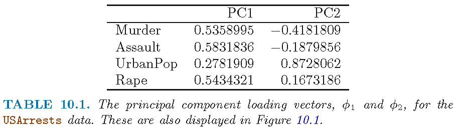
Total variability revisited
Recall \((d_i,\tilde{\mathbf{v}}_i)\) is an eigenpair for \(\tilde{\mathbf{S}}=\tilde{\mathbf{X}}^T\tilde{\mathbf{X}}\) that has eigenvalues \(d_1 \ge \cdots \ge d_p>0\)
- Recall \(\tilde{\mathbf{z}}_i = \tilde{\mathbf{X}} \tilde{\mathbf{v}}_i\) and that \(d_i=\Vert \tilde{\mathbf{z}}_i \Vert^2\) are the successive maximal variabilities of \(\tilde{\mathbf{X}}\) along any set of \(p\) orthonormal directions
Recall total variability of standardized data \(\tilde{\mathbf{X}}\) as \[ \sigma_{\text{total}}^2=\sum\nolimits_{i=1}^n \sum\nolimits_{j=1}^p \tilde{x}_{ij}^2 = (n-1)p \]
Caution: for a data matrix \(\mathbf{X}=(x_{ij}) \in \mathbb{R}^{n \times p}\) that is not necessarily centered or scaled, the total variability is \[ \sigma_{\text{total}}^2=\sum\nolimits_{i=1}^n \sum\nolimits_{j=1}^p {x}_{ij}^2 \]
Proportion of variance explained
For PCA on \(\mathbf{X}=(x_{ij}) \in \mathbb{R}^{n \times p}\),
- the “proportion of variance explained (PVE)” by the \(i\)-th principal component (i.e., PC) is defined as \(\tau_i=d_i/\sigma_{\text{total}}^2\)
- the “cumulative proportion of variance explained (CPVE)” by the first \(q\) PCs is defined as \[ T_q = (1/\sigma_{\text{total}}^2){\sum_{i=1}^q d_i}={\sum_{i=1}^q \tau_i}, \]
where \((d_i,\tilde{\mathbf{v}}_i)\) is an eigenpair of \({\mathbf{S}}={\mathbf{X}}^T{\mathbf{X}}\) that has eigenvalues \(d_1 \ge \cdots \ge d_r>0\) and \(r=\text{rank}(\mathbf{X})\)
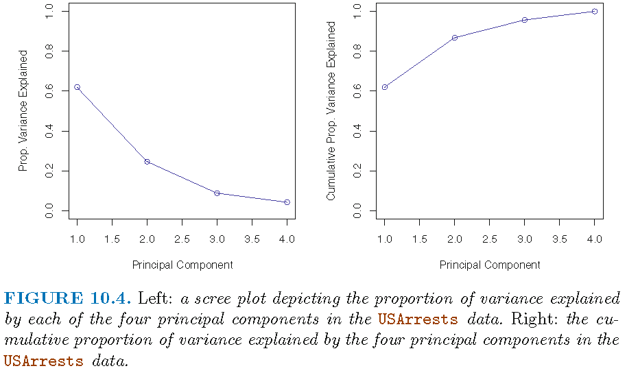
Variance explained
(Cumulative) Proportion of variance explained by subspaces of different dimensions
> # standardized data
> Xsd = scale(USArrests,center=TRUE,scale=TRUE)
> sum(Xsd^2) # total variability of standardized data
[1] 196
> pcaXsd = prcomp(Xsd) # PCA for standardized data
> pcaXsd$rotation # directions or loading vectors
                PC1        PC2        PC3         PC4
Murder   -0.5358995  0.4181809 -0.3412327  0.64922780
Assault  -0.5831836  0.1879856 -0.2681484 -0.74340748
UrbanPop -0.2781909 -0.8728062 -0.3780158  0.13387773
Rape     -0.5434321 -0.1673186  0.8177779  0.08902432
> # successive maximal lengths/variabilities of projections
> (nrow(USArrests)-1)*((pcaXsd$sdev)^2)
[1] 121.531837  48.498492  17.471596   8.498074
> # proportion of variance explained by each PC
> (nrow(USArrests)-1)*((pcaXsd$sdev)^2)/sum(Xsd^2)
[1] 0.62006039 0.24744129 0.08914080 0.04335752
> # cumulative proportion of variance explained
> cumsum((nrow(USArrests)-1)*((pcaXsd$sdev)^2))/sum(Xsd^2)
[1] 0.6200604 0.8675017 0.9566425 1.0000000
Plot of variance explained
(Cumulative) Proportion of variance explained
Patterns in data
- Often patterns in data are checked by plotting scores (i.e., projections), loadings (i.e., directions) of different PCs against each other in 2D or 3D
- We already discussed how to spot a dominant feature from a dominant entry in a loading vector
- Sometimes, other patterns can be spotted by adding observation labels to plot of scores
- A biplot plots both scores and loadings with observation labels
Cuation: PCA is not designed for the purpose of pattern recognition but rather for providing optimal orthogonal directions of successive maximal data variability
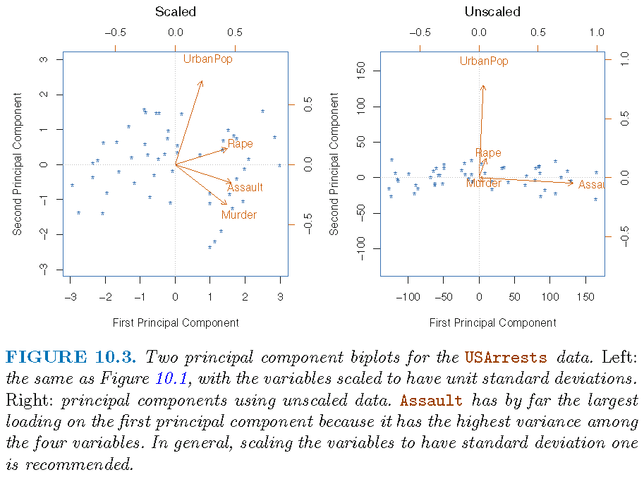
Biplot for PCA
In a biplot for PCA, there are 2 coordinate systems that share the same origin, such that
one coordinate system has \(x\)-coordinate for scores (i.e., entries of score vector) of PC \(i\) and \(y\)-coordinate for scores of another PC \(j\) and has the orientation and layout of the conventional \(x\)-\(y\) coordinate system
the other coordinate system has \(x\)-coordinate for loadings (i.e., entries of loading vector) of PC \(i\) and \(y\)-coordinate for loadings of another PC \(j\), where the \(x\)-axis tick marks are on the top and \(y\)-axis tick marks are on the right
Biplot for PCA
- “First/Second principal component” as “First/Second principal component score vector and loading vector”
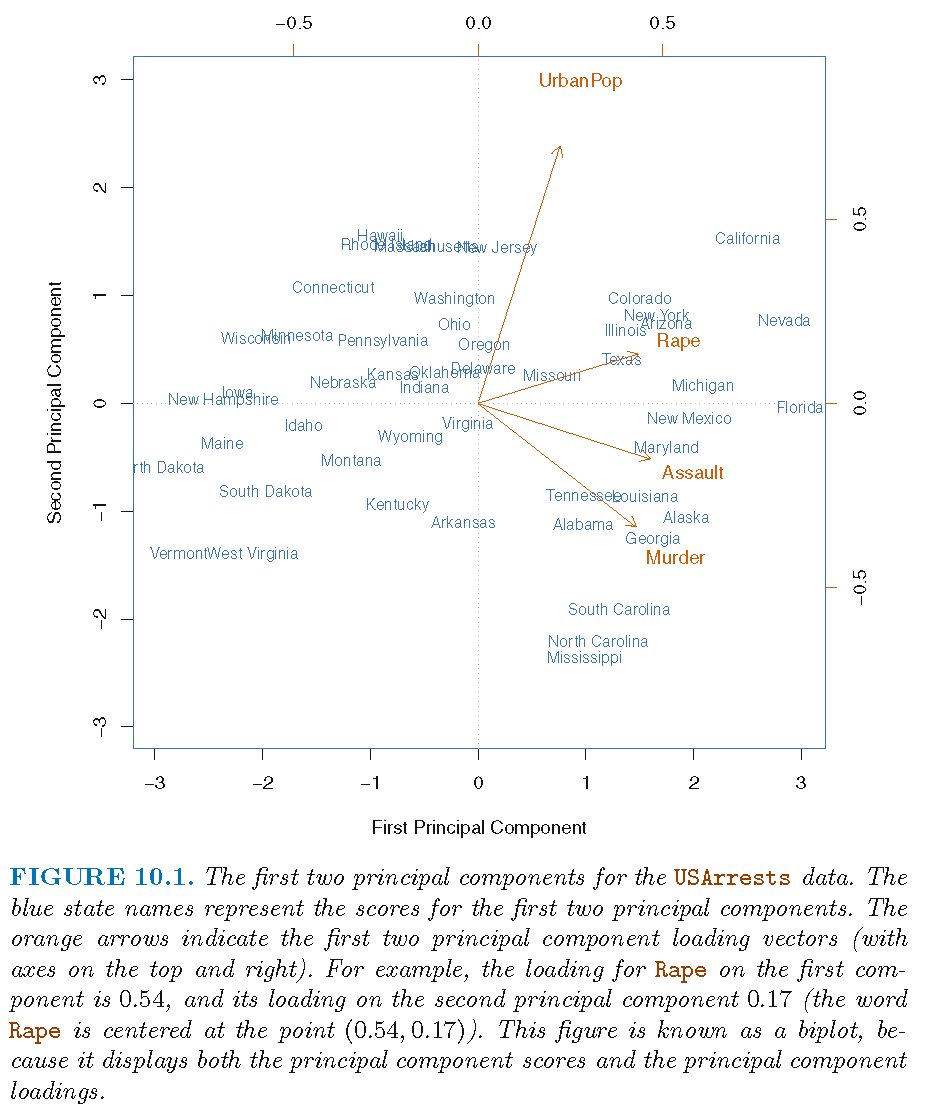
Findings from biplot
The first loading vector places approximately equal weight on
Assault,Murder, andRapebut much less weight onUrbanPop. So, the first PC roughly corresponds to a measure of overall rates of serious crimesThe second loading vector places most of its weight on
UrbanPopand much less weight on the other three featuresAssault,Murder, andRape. So, the second PC roughly corresponds to the level of urbanization of a state
Findings from biplot
Overall, crime-related variables (
Murder,Assault, andRape) are located close to each other, andUrbanPopvariable is far from these three crime-related variables. This indicates that the crime-related variables are correlated with each other (i.e., states with high murder rates tend to have high assault and rape rates) and thatUrbanPopvariable is less correlated with the three crime-related variables (Murder,Assault, andRape)The above finding is consistent with the correlation plot for the 4 features
Findings from biplot
We can examine differences between the US states via the two PC score and loading vectors via the biplot:
- States with large positive scores on the first PC, such as California, Nevada and Florida, have high crime rates
- States like North Dakota, with negative scores on the first PC, have low crime rates. California also has a high score on the second PC, indicating a high level of urbanization, while the opposite is true for states like Mississippi
- States close to zero on both PCs, such as Indiana, have approximately average levels of both crime and urbanization
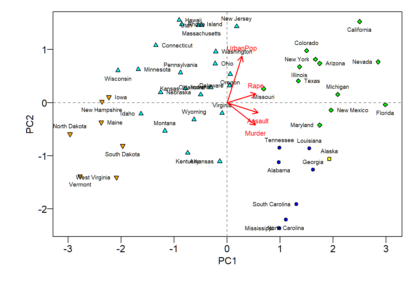
PCA biplot and clustering
5 clusters from hierarchical clustering, indicated by different shapes and superimposed on biplot; findings from biplot and clustering of states seem to be consistent with each other
Effects of scaling
Sample variance of each feature (where features are measured on different scales):
    Murder    Assault   UrbanPop       Rape
  18.97047 6945.16571  209.51878   87.72916
If PCA is applied to unscaled data,
- the 1st PC loading vector will place almost all of its weight on
Assaultsince it has the largest sample variance (that greatly dominates those of the other 3 features) - the 2nd PC loading vector will place almost all of its weight on
UrbanPop(since it has the second largest sample variance that considerably dominates those of the remaining 2 features)
Effects of scaling
We do not want results of PCA to be dependent on magnitudes of feature measurements
Pick the number of PCs
- For a column-centered data matrix \(\mathbf{X} \in \mathbb{R}^{n \times p}\), each of whose row is an observation on \(p\) linearly independent features, there are a maximum of \[r=\text{rank}(\mathbf{X})=\min\{n-1,p\}\] principal components (PCs)
- A general principle to choose the number of PCs is to choose a minimum number of PCs that together explain a given cumulative proportion of variance
- Cumulative proportion of variance explained for PCA on standardized data:
[1] 0.6200604 0.8675017 0.9566425 1.0000000An important connection
If we know covariance matrix \(\Sigma\) of feature vector \(X\), then we can implement population version PCA using spectral decomposition of \(\Sigma\), and project \(X\) onto orthonormal eigenvectors of \(\Sigma\) to achieve maximal successive explained variabilities
If we do not know \(\Sigma\), then we apply data version PCA using spectral decomposition of \(\mathbf{S}=\mathbf{X}^T \mathbf{X}\) if \(\mathbf{X}\) is column-centered since \(\mathbf{S}\) is proportional to sample covariance matrix \(\hat{\Sigma}\) of \(X\), and project each observation \(x_i\) onto orthonormal eigenvectors of \(\mathbf{S}\)
An important connection
Usually, orthonormal eigenvectors of \(\mathbf{S}=\mathbf{X}^T \mathbf{X}\) are regarded as an estimate (modulo \(\pm\) signs) of orthonormal eigenvectors of \(\Sigma\). So, data version PCA actually tries to estimate population version PCA in terms of principal components, directions and scores
When \(n \gg p\), this estimation is often very good, whereas when \(n \le p\), this estimation is often bad, and other ways (different than using spectral decomposition of sample covariance matrix) of estimating population version PCA should be used
Principal component analysis (PCA): Example 2
Human cancer microarray data
Human cancer data:
- 6830 genes (i.e., \(p=6830\) features) and their expressions
- 64 samples (i.e., \(64\) cancer cell lines)
- 14 different cancer types; information on cancer types at wiki-NCI60
We will pick observations for 3 caner types “BREAST”, “OVARIAN” and “LEUKEMIA”, and this gives a data matrix \(\mathbf{X} \in \mathbb{R}^{19 \times 6830}\)
PCA on high-dimensional data
Recall data matrix \(\mathbf{X} \in \mathbb{R}^{19 \times 6830}\), i.e., \(p=6830\) features and \(n=19\) samples/observations:
- once column centered and scaled, standardized data matrix \(\tilde{\mathbf{X}}\) has rank \(18\)
- PCA on \(\tilde{\mathbf{X}}\) can have a maximum of \(18\) PC’s, for which each loading vector is \(6830\)-dimensional and each score vector is \(19\)-dimensional
We are dealing with the so called “high-dimensional data”, where dimension reduction techniques such as PCA are even more important
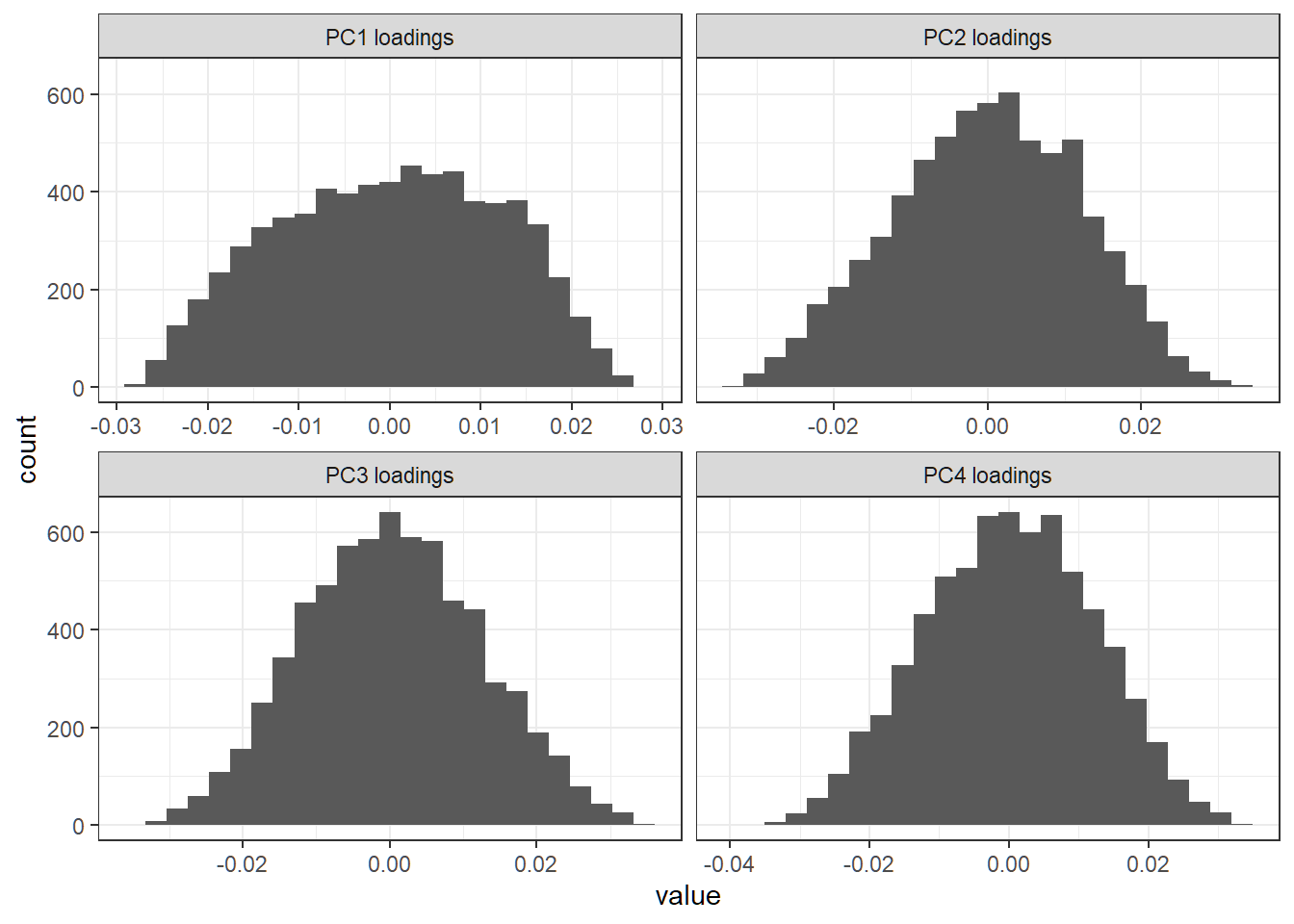
First 4 PC loading vectors
Each loading vector has a lot of nonzero entries; there seem to be no dominant features (i.e., genes) in any direction
Proportion of variance explained
Cumulative “PVE”:
 [1]  16.95366  27.33261  36.83971  44.15321  50.83002
 [6]  56.55363  62.01891  66.77877  71.51763  75.68344
[11]  79.67929  83.60823  87.38751  90.98552  94.09808
[16]  96.83802  99.13764 100.00000 100.00000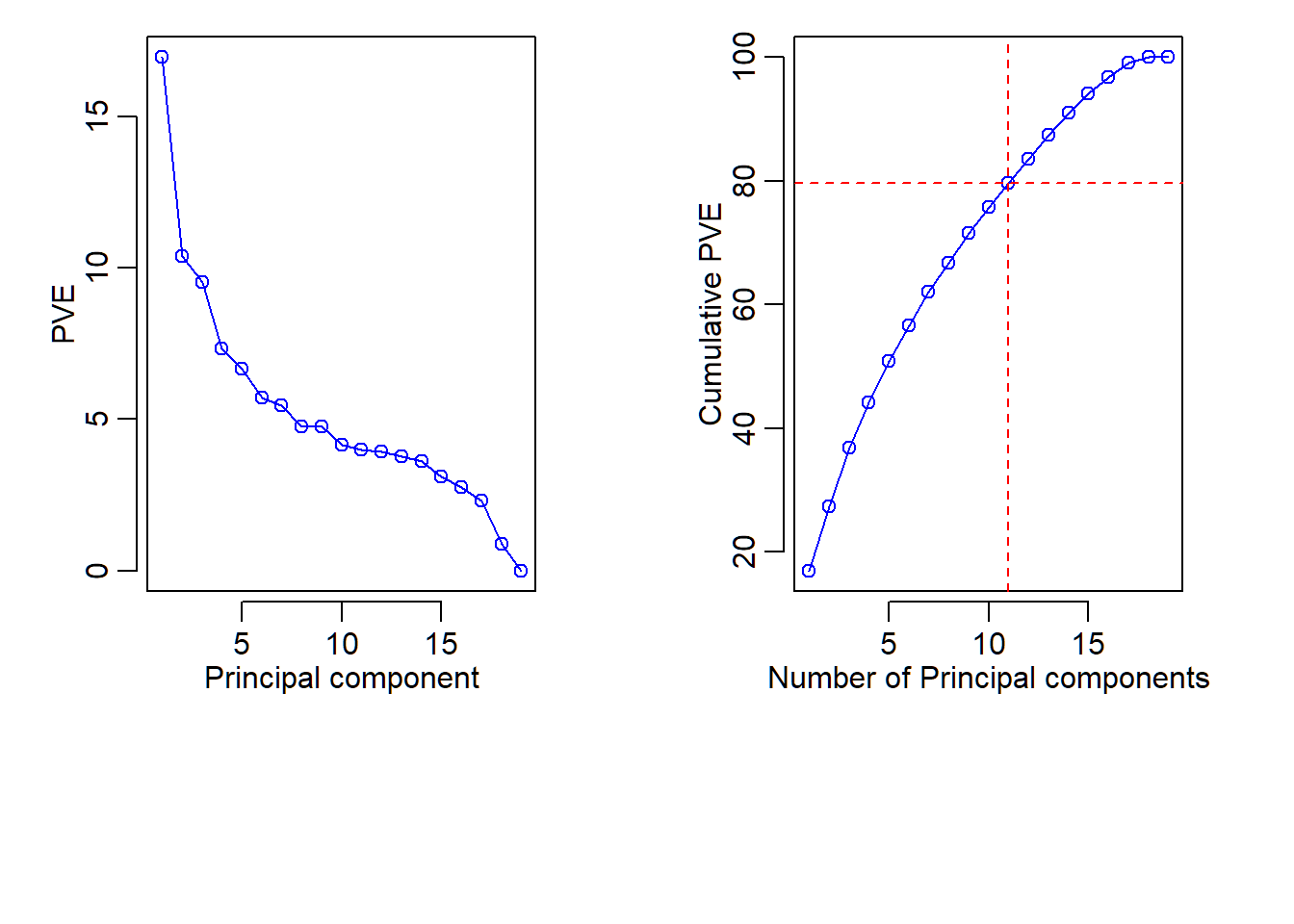
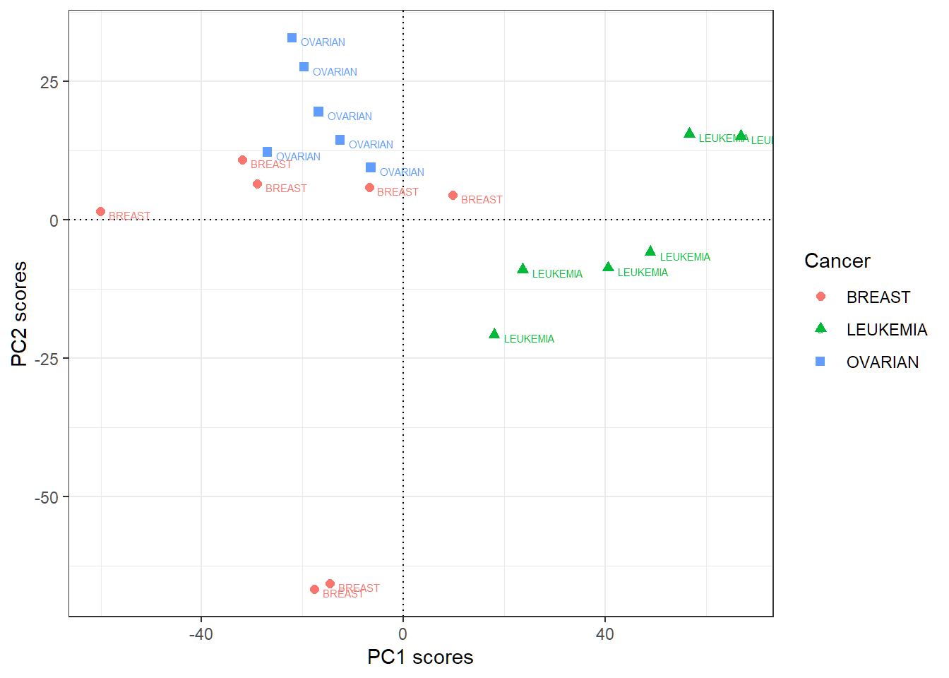
First 2 PC score vectors
- Rowname for row \(i\) of the score matrix (each of whose columns is a score vector) is the label (i.e., cancer type) for observation \(i\); “PC\(j\)” here means “score vector for PC\(j\)”
                PC1        PC2
BREAST   -60.098790   1.588815
BREAST   -31.889651  10.877669
BREAST   -29.035831   6.582595
OVARIAN  -19.721568  27.641286
OVARIAN  -12.608223  14.464804
OVARIAN  -26.962732  12.273994
OVARIAN   -6.453167   9.465530
OVARIAN  -22.091467  32.942808
OVARIAN  -16.828185  19.572828
LEUKEMIA  17.967827 -20.708967
LEUKEMIA  40.596818  -8.642872
LEUKEMIA  48.904273  -5.795735
LEUKEMIA  66.947137  15.148187
LEUKEMIA  56.697268  15.532885
LEUKEMIA  23.671867  -8.962769
BREAST     9.829156   4.542899
BREAST    -6.791608   5.910896
BREAST   -17.605215 -66.753270
BREAST   -14.527909 -65.681584
First 2 PC score vectors
Large positive PC1 scores indicative of “LEUKEMIA”, and large positive PC2 scores of “OVARIAN”
Sparse principal component analysis (SPCA)
Motivation: ordinary PCA
Recall standardized data matrix \(\tilde{\mathbf{X}} \in \mathbb{R}^{n \times p}\)
Recall spectral decomposition of \(\tilde{\mathbf{S}}=\tilde{\mathbf{X}}^T \tilde{\mathbf{X}}\) as \[ \tilde{\mathbf{S}}\tilde{\mathbf{v}}_i = d_i \tilde{\mathbf{v}}_i \iff \tilde{\mathbf{S}} = \mathbf{V} \mathbf{D} \mathbf{V}^T \] for an orthogonal matrix \(\mathbf{V}=(\tilde{\mathbf{v}}_1,\ldots,\tilde{\mathbf{v}}_p) \in \mathbb{R}^{p\times p}\) and a diagonal matrix \(\mathbf{D}=\text{diag}\{d_1,\ldots,d_p\}\) such that \[ d_1 \ge \cdots \ge d_{r} > 0 =d_{r+1} = \cdots = d_{p} = 0 \] when \(\tilde{\mathbf{X}}\) has rank \(r\)
PCA sets \(\tilde{\mathbf{z}}_i =\tilde{\mathbf{X}}\tilde{\mathbf{v}}_i\) for \(1 \le i \le r\), where \(\tilde{\mathbf{z}}_i\) and \(\tilde{\mathbf{v}}_i\) are the score vector and loading vector for the \(i\)-th PC, respectively
Motivation: dominant features
Let \(\tilde{\mathbf{v}}_i=(\phi_{i1},\ldots,\phi_{ip})^T\) for a fixed \(i\). Recall the following:
If the \(s\)-th entry \(\phi_{is}\) of \(\tilde{\mathbf{v}}_i\) has absolute value that dominates those of other entries of \(\tilde{\mathbf{v}}_i\), then the projection of observation \(\tilde{x}_r\) onto \(\tilde{\mathbf{v}}_i\) satisfies \(\tilde{z}_{ri} \approx \tilde{x}_{rs}\phi_{is}\)
- In this case, the projection of the standardized data matrix \(\tilde{\mathbf{X}}\) onto \(\tilde{\mathbf{v}}_i\) \[ \tilde{\mathbf{z}}_i \approx \phi_{is} \tilde{\mathbf{x}}_s, \] where \(\tilde{\mathbf{x}}_s\) is the \(s\)-th column of \(\tilde{\mathbf{X}}\) that contains \(n\) standardized observations for feature \(s\)
In this case, feature \(s\) contributes the dominant proportion of variation of standardized data \(\tilde{\mathbf{X}}\) along direction \(\tilde{\mathbf{v}}_i\)
Motivation: interpretability
If a majority of entries of a loading vector \(\tilde{\mathbf{v}}_i\) are zero, then we can easily identify dominant features along direction \(\tilde{\mathbf{v}}_i\), i.e., identify features that explain or account for most (or even all) of the variability of data \(\tilde{\mathbf{X}}\) along \(\tilde{\mathbf{v}}_i\)
However, for ordinary PCA, its PC’s are hard to interpret since each PC is a linear combination of all feature variables via a loading vector (i.e., coefficients of the linear combination are entries of a loading vector) and often a loading vector has many nonzero entries
Namely, for ordinary PCA, it is hard to identify a few features in a direction that accounts for most of the variability of data along that direction
Sparse PCA
- Sparse PCA aims to produce sparse loading vectors, i.e., loading vectors most of whose entries are zero, to enhance interpretability of PC’s in terms of dominant features along a direction
- Sparse PCA is a modification of ordinary PCA, such that its sparse loading vectors are still directions for projecting data matrix onto and are constrained, approximate directions for maximal successive variabilities of data, and that its score vectors are not necessarily uncorrelated
- To illustrate sparse PCA (SPCA), we will use some results from the paper “Sparse Principal Component Analysis” by Hui Zou, Trevor Hastie and Robert Tibshirani
Capture directions
- Assume data matrix \(\mathbf{X} \in \mathbb{R}^{n \times p}\) is standardized with \(x_{i}\) as its \(i\)th row
- Find optimizer \((\hat{\alpha},\hat{\beta})\) for the optimization problem \[\begin{equation} \min_{\alpha\in\mathbb{R}^{p\times q},\beta\in\mathbb{R}^{p\times q};\alpha^{T}\alpha=I_{q}} \sum_{i=1}^{n}\left\Vert x_{i}^T-\alpha\beta^{T} x_{i}^T\right\Vert^{2} +\lambda\sum_{j=1}^{q}\left\Vert \beta_{j}\right\Vert^{2}, \end{equation}\] where \(\beta_{j}\) is the \(j\)th column of \(\beta\) and \(\lambda >0\) is the tuning parameter. Note \(\alpha\) has \(q\) orthonormal columns
- Let \(\hat{\beta}_{i}\) be \(i\)-th column of \(\hat{\beta}\). Then \(\hat{\beta}_{i}=c_i\tilde{\mathbf{v}}_{i}\) for some \(c_i \in \mathbb{R}\), where \((d_i,\tilde{\mathbf{v}}_{i})\) is an eigenpair for \(\mathbf{S}=\mathbf{X}^T \mathbf{X}\)
- The optimization problem is called “ridge regression” due to the “\(l_2\)-penalty” on \(\beta\) as \(\lambda\sum_{j=1}^{q}\left\Vert \beta_{j}\right\Vert^{2}\)
Obtain sparse loadings
- Find optimizer of \((\hat{\alpha},\hat{\beta})\) for the optimization problem \[\begin{equation} \min_{\alpha\in\mathbb{R}^{p\times q},\beta\in\mathbb{R}^{p\times q};\alpha^{T}\alpha=I_{q}} \left\{\sum_{i=1}^{n}\left\Vert x_{i}^T-\alpha\beta^{T} x_{i}^T\right\Vert^{2} +\lambda\sum_{j=1}^{q}\left\Vert \beta_{j}\right\Vert^{2}\right.\\ \left. +\sum_{j=1}^{q}\lambda_{1,j}\left\Vert \beta_{j}\right\Vert_{1}\right\}, \end{equation}\] where \(\beta_{j}\) is the \(j\)th column of \(\beta\), \(\left\Vert \beta_{j}\right\Vert_{1}\) is the sum of absolute values of all entries of \(\beta_{j}\) (and is the called “\(l_1\)-norm” of \(\beta_{j}\)), and \(\lambda_{1,j}>0\) are tuning parameters
- The term \(\sum_{j=1}^{q}\lambda_{1,j}\left\Vert \beta_{j}\right\Vert_{1}\) is called the “\(l_{1}\)-penalty” for \(\beta\), and it sets some entries of \(\hat{\beta}=(\hat{\beta}_{1},\ldots,\hat{\beta}_{q})\) to be zero
SPCA: summary
The optimization problem in the previous slide is called an “elastic net regularization”, where
- the \(l_{2}\)-penalty attempts to capture directions (i.e., loading vectors) to project data onto
- the \(l_{1}\)-penalty sets some entries of each captured direction to be zero to produce sparse directions (i.e., sparse loading vectors) for better interpretability of PCs
- The optimal \(\hat{\beta}_{j} \in \mathbb{R}^p\) is the sparse loading vector and \(\tilde{\mathbf{z}}_j=\mathbf{X}\hat{\beta}_{j} \in \mathbb{R}^n\) the score vector respectively for sparse PC (SPC) \(j\) for \(j=1,\ldots,q\)
Caution: unlike ordinary PCA, the score vectors of SPCA are not necessarily uncorrelated
Data set
- The
pitpropsdata is a correlation matrix that was calculated from \(n=180\) observations on \(p=13\) features - This data set is the classic example showing the difficulty of interpreting ordinary PCs. The first 6 PCs will be examined
- In each of the tables to be given, the “Variance (%)” is the “percentage of variance explained (PVE)” by a PC and “Cumulative Variance (%)” the CPVE together by the corresponding PC’s
- Since score vectors of SPCA are not necessarily uncorrelated, PVE and CPVE for SPCA are computed differently than ordinary PCA and are called “adjusted” PVE and “adjusted” CPVE, respectively
Loadings from ordinary PCA
Loadings from sparse PCA
Overall a sparse PC explains a bit less variability than an ordinary PC but provides greater interpretability
Remarks
Since the
pitpropsdata is a correlation matrix but not a data matrix, a biplot cannot be created for SPCA in this setting. In general, a biplot cannot be created for PCA or SPCA if only a correlation or covariance matrix is availableWhen there are many features, a biplot may not be able to show loading vectors very clearly
Sparse principal component analysis (SPCA): Example 1
Human cancer microarray data
Human cancer data:
- 6830 genes (i.e., \(p=6830\) features) and their expressions
- 64 samples (i.e., \(64\) cancer cell lines)
- 14 different cancer types; information on cancer types at wiki-NCI60
We will pick observations for 3 caner types “BREAST”, “OVARIAN” and “LEUKEMIA”, and this gives a data matrix \(\mathbf{X} \in \mathbb{R}^{19 \times 6830}\)
SPCA on high-dimensional data
Recall data matrix \(\mathbf{X} \in \mathbb{R}^{19 \times 6830}\), i.e., \(p=6830\) features and \(n=19\) samples:
- once column centered and scaled, standardized data matrix \(\tilde{\mathbf{X}}\) has rank \(18\)
- SPCA on \(\tilde{\mathbf{X}}\) can have \(18\) SPC’s, for which each loading vector is \(6830\)-dimensional and each score vector is \(19\)-dimensional
- SPCA will be implemented with tuning parameter \(\lambda=10^{-6}\) for \(l_2\)-penalty and tuning parameters \(\lambda_{1,j}=10^{-6}\) for \(1 \le j \le 18\) for \(l_1\)-penalty to get 18 SPCs
- Caution: not easy to choose tuning parameters by cross-validation when \(n=19\) and \(p=6830\)
First 4 sparse loading vectors
Histogram of entries of a loading vector; each sparse loading vector has a lot of zero entries
First 4 ordinary loading vectors
Histogram of entries of a loading vector; each ordinary loading vector has a lot of nonzero entries

Adjusted PVE and CPVE
- Since SPCA is based on penalized regression, “cumulative proportion of variance explained (CPVE)” by all designated SPCs is not necessarily equal to the total variability of data
- Instead, CPVE of a set of designated SPCs for SPCA is the value of the quadratic term (involving data matrix) in the objective function (in the elastic net regularization) that is evaluated at the optimizer, and the optimizer depends on tuning parameters and the specified number of sparse PCs to compute
- Since score vectors in SPCA are not necessarily uncorrelated, PVE and CPVE are computed differently than ordinary PCA and are called adjusted PVE and adjusted CPVE
Ajusted PVE and CPVE
18 sparse PCs in total and adjusted CPVE:
 [1] 0.04121285 0.06446548 0.08576216 0.10116359 0.11575015
 [6] 0.12716561 0.13836691 0.14794329 0.15798456 0.16611261
[11] 0.17404920 0.18198781 0.18927400 0.19637057 0.20227463
[16] 0.20750115 0.21207035 0.21387115
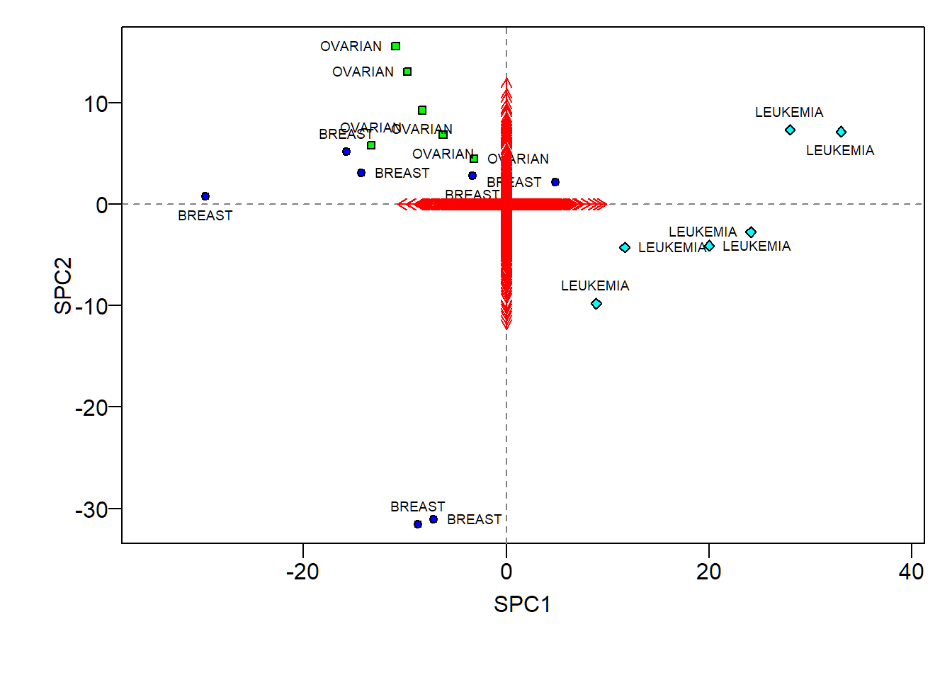
SPCA biplot
- Sparse loadings (scaled up 100 times) hard to visualize
- Large positive SPC1 scores indicative of “LEUKEMIA”, and large positive SPC2 scores of “OVARIAN”
License and session Information
> sessionInfo()
R version 3.5.0 (2018-04-23)
Platform: x86_64-w64-mingw32/x64 (64-bit)
Running under: Windows 10 x64 (build 19041)

Matrix products: default

locale:
[1] LC_COLLATE=English_United States.1252
[2] LC_CTYPE=English_United States.1252
[3] LC_MONETARY=English_United States.1252
[4] LC_NUMERIC=C
[5] LC_TIME=English_United States.1252

attached base packages:
[1] stats     graphics  grDevices utils     datasets  methods
[7] base

other attached packages:
[1] knitr_1.21

loaded via a namespace (and not attached):
 [1] compiler_3.5.0  magrittr_1.5    tools_3.5.0
 [4] htmltools_0.3.6 revealjs_0.9    yaml_2.2.0
 [7] Rcpp_1.0.0      stringi_1.2.4   rmarkdown_1.11
[10] stringr_1.3.1   xfun_0.4        digest_0.6.18
[13] evaluate_0.12