R software and commands

R libraries and commands needed:

• R built-in command prcomp{stats} to implement PCA
• R built-in command biplot.princomp{stats} to create biplot for PCA

Command prcomp

• prcomp{stats} performs PCA on a data matrix and returns the results as an object of class prcomp

• The calculation is done by a singular value decomposition (SVD) of the (centered and possibly scaled) data matrix but not by using the command eigen on the covariance matrix. This is generally the preferred method for numerical accuracy. The print method for these objects prints the results in a nice format, and the plot method produces a scree plot

Command prcomp

The basic syntax of prcomp{stats} is:

prcomp(x, retx = TRUE, center = TRUE, scale. = FALSE,
       tol = NULL, rank. = NULL, ...)

• x: a numeric or complex matrix (or data frame) which provides the data for PCA.
• retx: a logical value indicating whether the rotated variables (i.e., score vectors) should be returned.
• center: a logical value indicating whether the variables (i.e., features) should be shifted to be zero centered. Alternately, a vector of length equal the number of columns of x can be supplied. The value is passed to scale.

Command prcomp

Basic syntax:

prcomp(x, retx = TRUE, center = TRUE, scale. = FALSE,
       tol = NULL, rank. = NULL, ...)

• scale.: a logical value indicating whether the variables should be scaled to have unit variance before the analysis takes place. The default is FALSE but in general scaling is advisable. Alternatively, a vector of length equal the number of columns of x can be supplied. The value is passed to scale.

Command prcomp

Basic syntax:

prcomp(x, retx = TRUE, center = TRUE, scale. = FALSE,
       tol = NULL, rank. = NULL, ...)

• tol: a value indicating the magnitude below which principal components (PCs) should be omitted. PCs are omitted if their standard deviations (i.e., if the Euclidean norms of their score vectors) are less than or equal to tol times the standard deviation of the first PC. The default is null and no components are omitted (unless rank. is specified less than min(dim(x)). Also, tol=0 or tol=sqrt(.Machine$double.eps) can be set, which would omit essentially constant PCs.

Command prcomp

Basic syntax:

prcomp(x, retx = TRUE, center = TRUE, scale. = FALSE,
       tol = NULL, rank. = NULL, ...)

• rank.: a number specifying the maximal rank, i.e., maximal number of principal components to be used. It can be set as an alternative to or in addition to tol, and is useful notably when the desired rank is considerably smaller than the dimensions of the matrix x.

Command prcomp

prcomp returns a list with class “prcomp” containing the following components:

• sdev: a vector of standard deviations of PCs; the \(i\)-th entry of sdev is for PC \(i\). So, when x is column-centered, (nrow(x)-1)*(sdev^2) are the eigenvalues of t(x)%*%x, and their sum is the total variability for data in the column-centered x.

• rotation: matrix of loading vectors, i.e., the matrix whose columns are eigenvectors of t(x)%*%x when x is column-centered (and column-scaled).

Command prcomp

prcomp returns a list with class “prcomp” containing the following components:

• x: if retx=TRUE, then the value of the rotated data is returned, i.e., if retx=TRUE, x is the centered (and scaled if requested) data multiplied by the rotation matrix, i.e., if retx=TRUE, x is the matrix whose columns are score vectors. The \(i\)-th column of x pairs with the \(i\)-th column of rotation, and both are for PC \(i\).
• center and scale: the centering and scaling used if center=TRUE and scale.=TRUE; otherwise, either or both are FALSE.

Command biplot.princomp

biplot.princomp{stats} (i.e., biplot{stats} when applied to an object of class “prcomp” ) produces a biplot from the output of command prcomp (or princomp). Its basic syntax is:

biplot(x,choices = 1:2,scale = 1,pc.biplot=FALSE,cex=1,...)

• x: an object of class “prcomp” (or “princomp” whose details are given in Appendix 1).
• choices: a length 2 vector specifying the principal components to plot.
• cex: font size if biplot is annotated by labels of observations.

Command biplot.princomp

Basic syntax:

biplot(x,choices = 1:2,scale = 1,pc.biplot=FALSE,cex=1,...)

• scale: variables are scaled by lambda^scale and observations by lambda^(1-scale), where lambda are the singular values as computed by princomp. Normally 0 <= scale <= 1, and a warning will be issued if the specified scale is outside this range. By default, scale=1.
• pc.biplot: if true, use what Gabriel (1971) refers to as a “principal component biplot”, with lambda=1 and observations scaled up by sqrt(n) and variables scaled down by sqrt(n).

US arrests data

The USArrests data set (included in the library ISLR or ggplot2) contains arrests per 100,000 residents in each of the 50 US states in 1973. There are

• 4 features: 3 types of crimes Murder, Assault, Rape, and UrbanPop (percent of population living in urban areas)

> library(ISLR); dim(USArrests)
[1] 50  4
> head(USArrests)
           Murder Assault UrbanPop Rape
Alabama      13.2     236       58 21.2
Alaska       10.0     263       48 44.5
Arizona       8.1     294       80 31.0
Arkansas      8.8     190       50 19.5
California    9.0     276       91 40.6
Colorado      7.9     204       78 38.7

Correlations among features

• addCoef.col="grey": add correlation coefficient with color; tl.cex=0.57: font size for variables

> corMatFeature = cor(USArrests); library(corrplot)
> corrplot(corMatFeature,method="shade",addCoef.col="grey",
+          tl.cex=0.57, mar = c(4.5,1,1,1))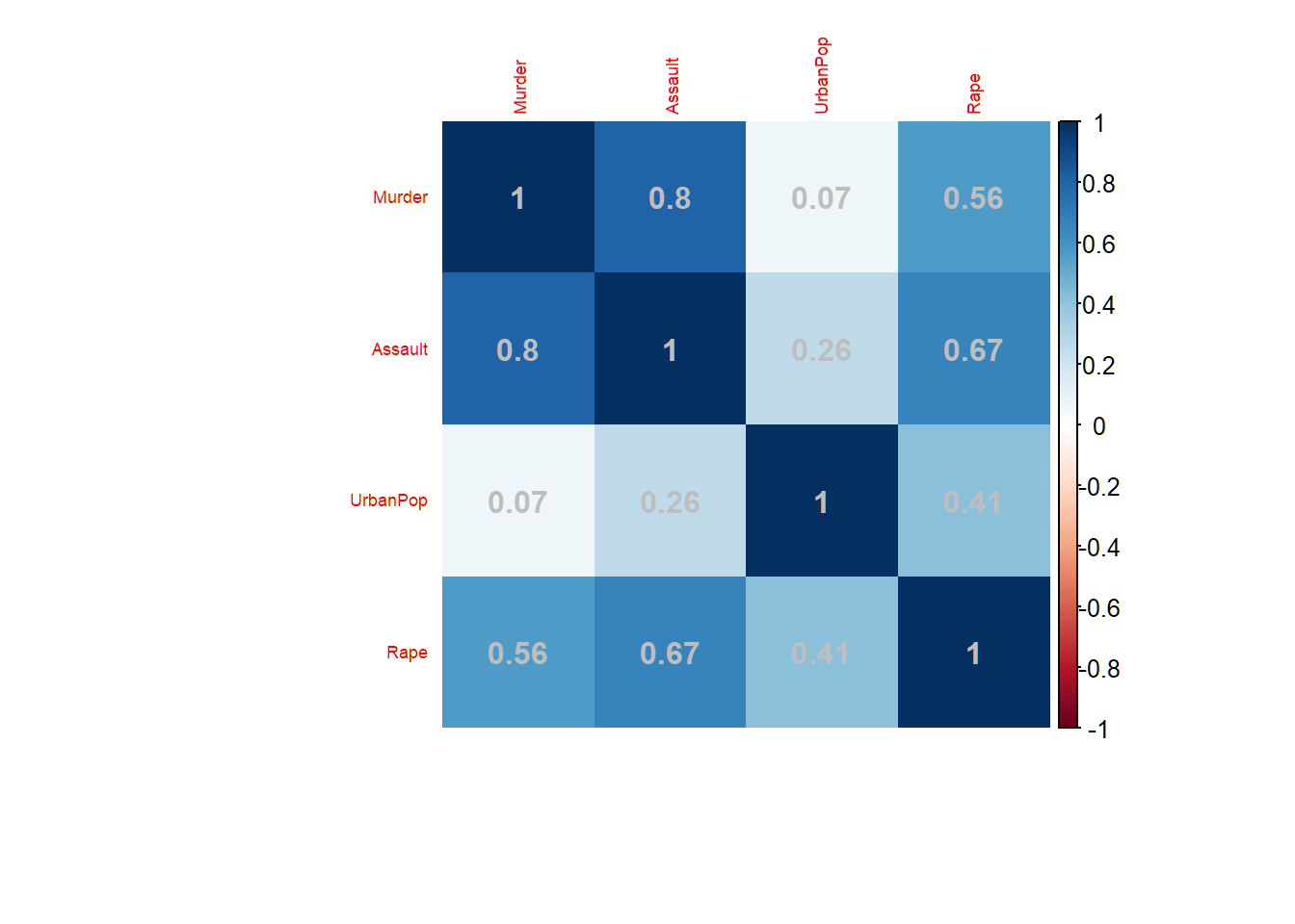

Dendrogram

> library(ggdendro); library(ggplot2)
> Xsd=scale(USArrests,center=TRUE,scale=TRUE)
> hc=hclust(dist(Xsd),"ave"); source("C:\\MathRepo\\stat437Online\\Plotggdendro.r")
> plot_ggdendro(dendro_data_k(hc,5),direction ="tb",expand.y = 0.2)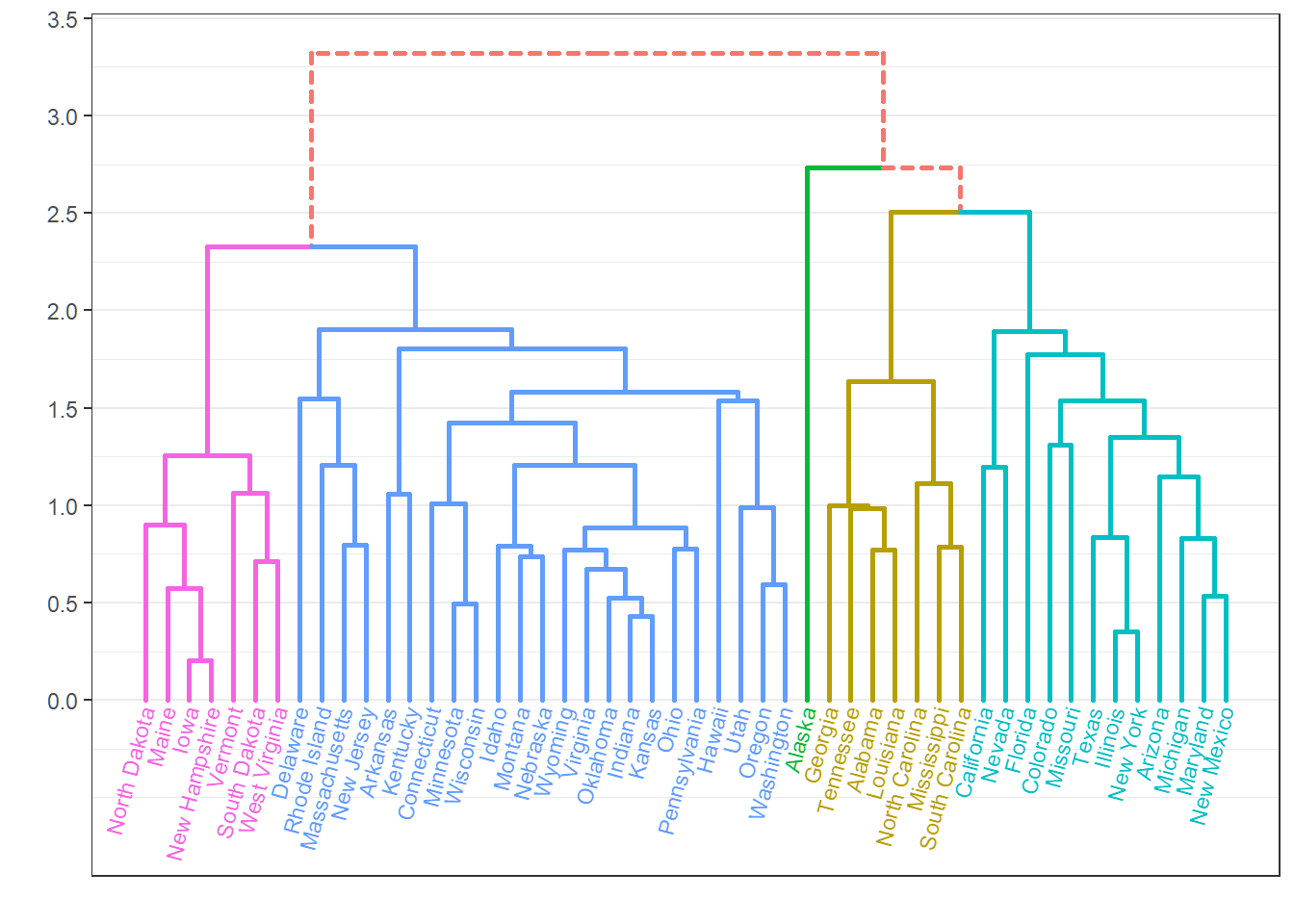

PCA of standardized data

• Acronym “PC” means “loading vector”

> # standardize data
> Xsd = scale(USArrests,center=TRUE,scale=TRUE)
> # total variability of standardized data
> sum(Xsd^2)
[1] 196
> # PCA for standardized data
> pcaXsd = prcomp(Xsd)
> # directions or loading vectors
> pcaXsd$rotation
                PC1        PC2        PC3         PC4
Murder   -0.5358995  0.4181809 -0.3412327  0.64922780
Assault  -0.5831836  0.1879856 -0.2681484 -0.74340748
UrbanPop -0.2781909 -0.8728062 -0.3780158  0.13387773
Rape     -0.5434321 -0.1673186  0.8177779  0.08902432
> # successive maximal variabilities of projections
> (nrow(USArrests)-1)*((pcaXsd$sdev)^2)
[1] 121.531837  48.498492  17.471596   8.498074
> # cumulative proportion of variance explained
> cumsum((nrow(USArrests)-1)*((pcaXsd$sdev)^2))/sum(Xsd^2)
[1] 0.6200604 0.8675017 0.9566425 1.0000000

• Note (nrow(USArrests)-1)*((pcaXsd$sdev)^2)

Score matrix

• Score matrix is \(n \times p\); each column is a score vector
• Each row is labelled by observation label

> options(digits=5)
> pcaXsd$x
                     PC1       PC2       PC3        PC4
Alabama        -0.975660  1.122001 -0.439804  0.1546966
Alaska         -1.930538  1.062427  2.019500 -0.4341755
Arizona        -1.745443 -0.738460  0.054230 -0.8262642
Arkansas        0.139999  1.108542  0.113422 -0.1809736
California     -2.498613 -1.527427  0.592541 -0.3385592
Colorado       -1.499341 -0.977630  1.084002  0.0014502
Connecticut     1.344992 -1.077984 -0.636793 -0.1172787
Delaware       -0.047230 -0.322089 -0.711410 -0.8731133
Florida        -2.982760  0.038834 -0.571032 -0.0953170
Georgia        -1.622807  1.266088 -0.339018  1.0659745
Hawaii          0.903484 -1.554676  0.050272  0.8937332
Idaho           1.623319  0.208853  0.257190 -0.4940879
Illinois       -1.365052 -0.674988 -0.670686 -0.1207949
Indiana         0.500381 -0.150039  0.225763  0.4203976
Iowa            2.230996 -0.103008  0.162910  0.0173795
Kansas          0.788872 -0.267449  0.025296  0.2044210
Kentucky        0.743313  0.948807 -0.028084  0.6638172
Louisiana      -1.549091  0.862300 -0.775606  0.4501578
Maine           2.372740  0.372609 -0.065022 -0.3271385
Maryland       -1.745647  0.423357 -0.155670 -0.5534506
Massachusetts   0.481280 -1.459677 -0.603372 -0.1777939
Michigan       -2.087250 -0.153835  0.381000  0.1013431
Minnesota       1.675670 -0.625907  0.151532  0.0666403
Mississippi    -0.986479  2.369737 -0.733363  0.2133420
Missouri       -0.689784 -0.260708  0.373650  0.2235548
Montana         1.173538  0.531479  0.244408  0.1224986
Nebraska        1.252916 -0.192004  0.173809  0.0157332
Nevada         -2.845505 -0.767805  1.151688  0.3113544
New Hampshire   2.359956 -0.017901  0.036485 -0.0328043
New Jersey     -0.179741 -1.434937 -0.756770  0.2409366
New Mexico     -1.960124  0.141413  0.181846 -0.3361211
New York       -1.665667 -0.814911 -0.636612 -0.0133488
North Carolina -1.112088  2.205611 -0.854892 -0.9447896
North Dakota    2.962152  0.593097  0.298249 -0.2514346
Ohio            0.223694 -0.734778 -0.030826  0.4691528
Oklahoma        0.308649 -0.284961 -0.015156  0.0102285
Oregon         -0.058528 -0.535970  0.930387 -0.2353909
Pennsylvania    0.879487 -0.565361 -0.396602  0.3554524
Rhode Island    0.855091 -1.476983 -1.356177 -0.6074027
South Carolina -1.307450  1.913973 -0.297517 -0.1301454
South Dakota    1.967797  0.815068  0.385381 -0.1084705
Tennessee      -0.989694  0.851605  0.186193  0.6463027
Texas          -1.341518 -0.408335 -0.487123  0.6367311
Utah            0.545032 -1.456715  0.290776 -0.0814867
Vermont         2.773256  1.388194  0.832808 -0.1434337
Virginia        0.095367  0.197728  0.011595  0.2092464
Washington      0.214723 -0.960374  0.618591 -0.2186282
West Virginia   2.087393  1.410526  0.103722  0.1305831
Wisconsin       2.058812 -0.605125 -0.137469  0.1822534
Wyoming         0.623101  0.317787 -0.238240 -0.1649769

Biplot for PCA

> # use reflection to comply with Textbook
> pcaXsd$rotation = -pcaXsd$rotation; pcaXsd$x = -pcaXsd$x
> par(mar=c(7,4.5,1.5,1),mgp=c(1.5,0.5,0))
> biplot(pcaXsd,choices=1:2,scale=1,pc.biplot=T,cex=0.5)
> # `cex=0.5`: font size for text labels
> abline(v=0, lty=2, col="grey50")
> abline(h=0, lty=2, col="grey50")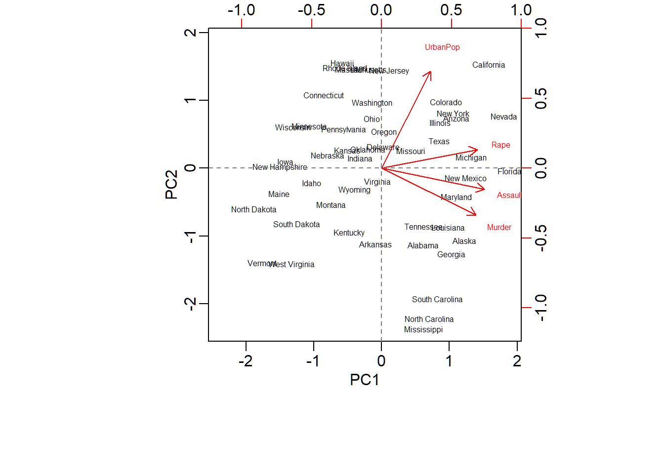

Customized biplot

Cluster memberships of US states superimposed on biplot of PCA of USArrests data

Remark on prcomp

• Let \(\tilde{\mathbf{X}} \in \mathbb{R}^{n \times p}\) be the standardized data matrix that is obtained from the data matrix \({\mathbf{X}} \in \mathbb{R}^{n \times p}\)

• The prcomp$sdev are square roots of the eigenvalues of the matrix \(\hat{\mathbf{X}}^T\hat{\mathbf{X}}\) with \[ \hat{\mathbf{X}}=(n-1)^{-1/2}\tilde{\mathbf{X}}, \] such that \(\text{tr}(\hat{\mathbf{X}}^T\hat{\mathbf{X}})=p\)

• \(\tilde{\mathbf{X}}^T\tilde{\mathbf{X}}\) and \(\hat{\mathbf{X}}^T\hat{\mathbf{X}}\) have the same set of orthonormal eigenvectors (modulo \(\pm\) signs ) but the eigenvalues of \(\tilde{\mathbf{X}}^T\tilde{\mathbf{X}}\) are \(n-1\) times those of \(\hat{\mathbf{X}}^T\hat{\mathbf{X}}\) when both sets of eigenvalues are arranged in descending order

Human cancer microarray data

Human cancer data:

• 6830 genes (i.e., \(p=6830\) features) and their expressions
• 64 samples (i.e., \(64\) cancer cell lines)
• 14 different cancer types; information on cancer types at wiki-NCI60

We will pick observations for 3 caner types “BREAST”, “OVARIAN” and “LEUKEMIA”, and this gives the uncentered data matrix \(\mathbf{X} \in \mathbb{R}^{19 \times 6830}\) (i.e., \(p=6830\) features and \(n=19\) observations)

PCA on standardized data

> library(ISLR); 
> nci.labs = NCI60$labs # cancer types or cell lines
> nci.data = NCI60$data # expression data matrix
> # pick 3 cancer types: BREAST, OVARIAN, LEUKEMIA
> nci.labs1 = nci.labs[nci.labs %in% 
+                 c('BREAST', 'OVARIAN', 'LEUKEMIA')]
> nci.data1 = nci.data[nci.labs %in% 
+                 c('BREAST', 'OVARIAN', 'LEUKEMIA'),]
> # standardize data
> Xsd = scale(nci.data1,center=TRUE,scale=TRUE)
> # PCA for standardized data
> pcaXsd = prcomp(Xsd)
> names(pcaXsd)
[1] "sdev"     "rotation" "center"   "scale"    "x"       
> dim(nci.data) # dimensions of data matrix
[1]   64 6830
> dim(pcaXsd$rotation) # dimensions of loading matrix
[1] 6830   19
> dim(pcaXsd$x) # dimensions of score matrix
[1] 19 19

Remarks on rank.

• In previous slide, \(19\) PCs, \(19\) loading vectors and \(19\) score vectors were produced because we used tol=NULL and rank.=NULL in command prcomp, which removed no PCs

• However, the \(19\)-th PC and its loading vector and score vector theoretically should not exist at all (since PCA was applied to the standardized data matrix \(\tilde{\mathbf{X}}\) which has rank \(18=\text{rank}(\tilde{\mathbf{X}})\)) but are by-products of machine precision. We can use rank.=18 to remove them.

• Since we did not remove any PC, the \(19\) PCs and their loading and score vectors, their PVEs and CPVE will appear in later slides (as illustrations for instruction)

Remarks on rank.

• In practice, we need to specify argument rank. to be \(\text{rank}(\tilde{\mathbf{X}})\) (i.e., the rank of \(\tilde{\mathbf{X}}\)) for command prcomp

• For the standardized data matrix \(\tilde{\mathbf{X}} \in \mathbb{R}^{n \times p}\) that contains \(n\) linearly independent observations on \(p\) linearly independent features (,which is usually the case), its rank \[\text{rank}(\tilde{\mathbf{X}}) = \min\{n-1,p\}.\] Namely, for such \(\tilde{\mathbf{X}}\), we set rank. to be \(\min\{n-1,p\}\) for prcomp

Obtain \(r=\text{rank}(\tilde{\mathbf{X}})\) PCs

• Standardized data matrix \(\tilde{\mathbf{X}}\) has rank \(r=18\), allowing for a maximum of \(18\) PCs when PCA is applied to \(\tilde{\mathbf{X}}\):

> library(ISLR); nci.labs = NCI60$labs; nci.data = NCI60$data
> nci.labs1 = nci.labs[nci.labs %in% 
+                 c('BREAST', 'OVARIAN', 'LEUKEMIA')]
> nci.data1 = nci.data[nci.labs %in% 
+                 c('BREAST', 'OVARIAN', 'LEUKEMIA'),]
> Xsd = scale(nci.data1,center=TRUE,scale=TRUE)
> # PCA for standardized data
> pcaXsd1 = prcomp(Xsd,rank.=nrow(nci.data1)-1)
> dim(nci.data) # dimensions of data matrix
[1]   64 6830
> dim(pcaXsd1$rotation) # dimensions of loading matrix
[1] 6830   18
> dim(pcaXsd1$x) # dimensions of score matrix
[1] 19 18
> cumsum(100*(nrow(nci.data1)-1)*pcaXsd1$sdev^2)/sum(Xsd^2) # CPVE
 [1]  16.95366  27.33261  36.83971  44.15321  50.83002
 [6]  56.55363  62.01891  66.77877  71.51763  75.68344
[11]  79.67929  83.60823  87.38751  90.98552  94.09808
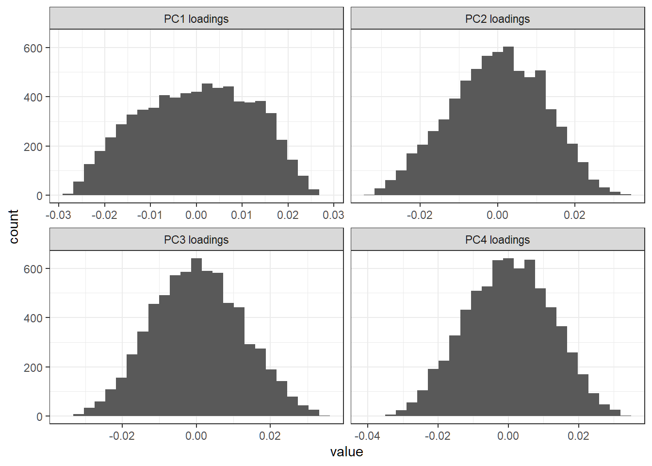
[16]  96.83802  99.13764 100.00000 100.00000

First 4 PC loading vectors

Create a histogram for entries of each of first 4 PC loading vectors:

> library(ggplot2); library(reshape2)
> # column names of loading matrix
> colnames(pcaXsd$rotation)
 [1] "PC1"  "PC2"  "PC3"  "PC4"  "PC5"  "PC6"  "PC7"  "PC8" 
 [9] "PC9"  "PC10" "PC11" "PC12" "PC13" "PC14" "PC15" "PC16"
[17] "PC17" "PC18" "PC19"
> # store first 4 PC loading vectors in a matrix
> FourLD = pcaXsd$rotation[,1:4]
> # change column names of `FourLD`
> colnames(FourLD)=paste(colnames(FourLD),"loadings",sep=" ")
> colnames(FourLD)
[1] "PC1 loadings" "PC2 loadings" "PC3 loadings" "PC4 loadings"
> # melt the matrix `FourLD` for plotting
> dstack <- melt(FourLD)
> # create a histogram for entries of each loading vector
> lvPlot=ggplot(dstack,aes(x = value))+
+   geom_histogram(bins = 25)+
+   facet_wrap(~Var2,scales = "free_x")+theme_bw()

First 4 PC loading vectors

Each loading vector has a lot of nonzero entries; there seem to be no dominant features (i.e., genes) in any direction

Proportion of variance explained

> # compute PVE for each PC; scaling (n-1) cancelled in ratio
> pve = 100*pcaXsd$sdev^2/sum(pcaXsd$sdev^2)
> pve
 [1] 1.695366e+01 1.037896e+01 9.507100e+00 7.313498e+00
 [5] 6.676814e+00 5.723603e+00 5.465282e+00 4.759858e+00
 [9] 4.738859e+00 4.165811e+00 3.995856e+00 3.928936e+00
[13] 3.779277e+00 3.598014e+00 3.112560e+00 2.739935e+00
[17] 2.299622e+00 8.623618e-01 2.256130e-29
> # compute cumulative PVE (CPVE)
> cumsum(pve)
 [1]  16.95366  27.33261  36.83971  44.15321  50.83002
 [6]  56.55363  62.01891  66.77877  71.51763  75.68344
[11]  79.67929  83.60823  87.38751  90.98552  94.09808
[16]  96.83802  99.13764 100.00000 100.00000

• The last, i.e., \(19\)-th, PVE should be theoretically \(0\) (since the standardized data matrix has rank \(18\)) but is numerically nonzero as 2.256130e-29 due to machine precision. However, it is essentially \(0\)

Plot of PVE and CPVE

> par(mfrow=c(1,2),mar=c(9,4,1,3),mgp=c(1.8,0.6,0.3))
> plot(1:length(pve), pve,type="o",ylab="PVE",
+      xlab="Principal component",col="blue")
> plot(cumsum(pve),type="o",ylab="Cumulative PVE",
+      xlab="Number of first PCs",col="blue")
> abline(h = cumsum(pve)[11], col="red", lty=2)
> abline(v = 11, col="red", lty=2)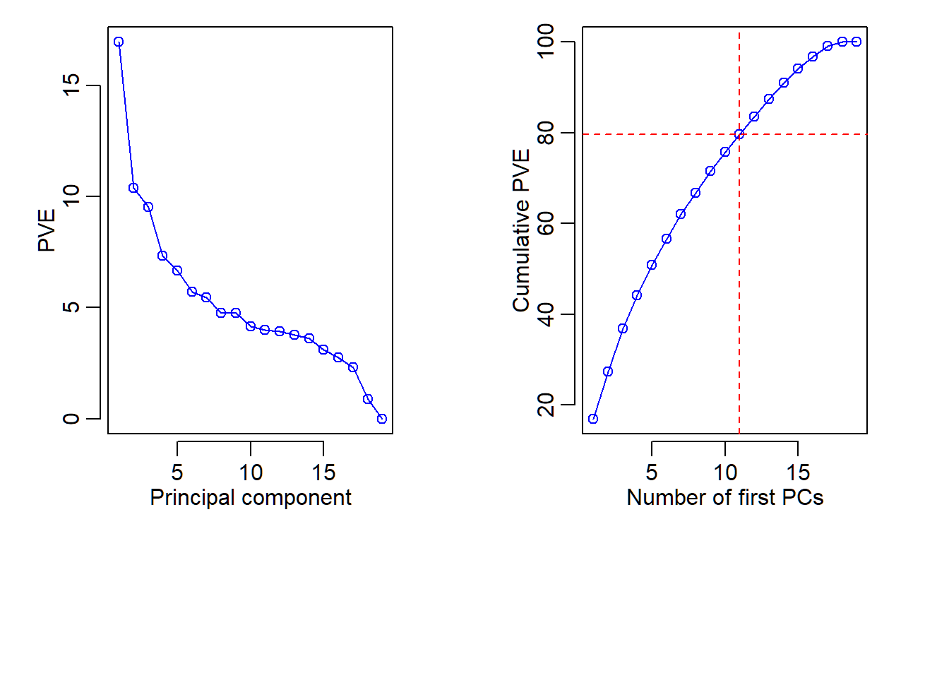

First 2 PC score vectors

• Data matrix does not have row names as cancer types
• Add rowname for row \(i\) of the score matrix (each of whose columns is a score vector) as the label (i.e., cancer type) for observation \(i\); “PC\(j\)” here means “score vector for PC\(j\)”

> scoresMat=as.data.frame(pcaXsd$x[,1:2])
> sMTmp=t(scoresMat); colnames(sMTmp)=nci.labs1
> scoresMat=t(sMTmp); scoresMat
                PC1        PC2
BREAST   -60.098790   1.588815
BREAST   -31.889651  10.877669
BREAST   -29.035831   6.582595
OVARIAN  -19.721568  27.641286
OVARIAN  -12.608223  14.464804
OVARIAN  -26.962732  12.273994
OVARIAN   -6.453167   9.465530
OVARIAN  -22.091467  32.942808
OVARIAN  -16.828185  19.572828
LEUKEMIA  17.967827 -20.708967
LEUKEMIA  40.596818  -8.642872
LEUKEMIA  48.904273  -5.795735
LEUKEMIA  66.947137  15.148187
LEUKEMIA  56.697268  15.532885
LEUKEMIA  23.671867  -8.962769
BREAST     9.829156   4.542899
BREAST    -6.791608   5.910896
BREAST   -17.605215 -66.753270
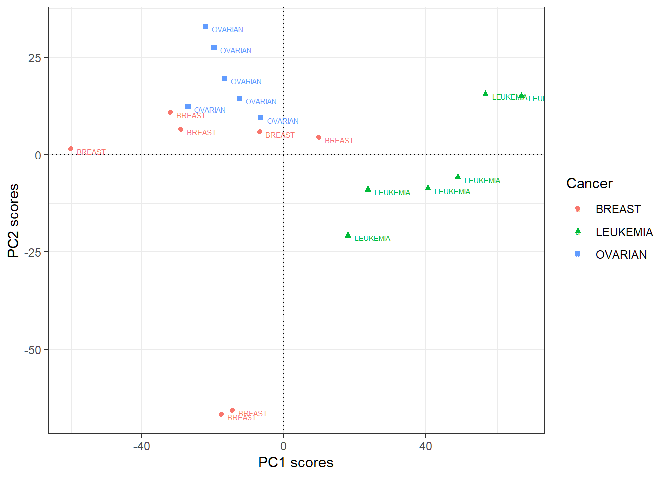
BREAST   -14.527909 -65.681584

Plot first 2 PC score vectors

> # store first 2 score vectors in a data.frame
> scoresMat=as.data.frame(pcaXsd$x[,1:2])
> # add cancer types for observations to be used as labels
> # when plotting scores
> scoresMat$Cancer=nci.labs1
> # create plot with `color=Cancer,shape=Cancer`
> library(ggplot2)
> pSV = ggplot(scoresMat,aes(PC1,PC2,
+                 color=Cancer,shape=Cancer))+
+   geom_point()+theme_bw()+xlab("PC1 scores")+
+   ylab("PC2 scores")+
+   geom_hline(yintercept = 0,linetype="dotted")+
+   geom_vline(xintercept = 0,linetype="dotted")+
+   geom_text(aes(label=Cancer),hjust=-0.2, vjust=0.9,size=2)
> # geom_hline and geom_vline as center lines as references

Plot first 2 PC score vectors

PC1 scores more indicative of “LEUKEMIA”, and PC2 scores of “OVARIAN”; other patterns may exist

R software and commands

R libraries and commands needed:

• R library elasticnet and its command spca for sparse PCA

Command spca

spca{elasticnet} implements SPCA using an alternating minimization algorithm to minimize the SPCA objective function. Its basic syntax is:

spca(x, K, para, type=c("predictor","Gram"),
     sparse=c("penalty","varnum"), use.corr=FALSE,
     lambda=1e-6,
     max.iter=200, trace=FALSE, eps.conv=1e-3)

• x: A matrix. It can be the predictor matrix or the sample covariance/correlation matrix.
• K: Number of principal components to compute.
• para: A vector of length K with all positive elements.

Command spca

Basic syntax:

spca(x, K, para, type=c("predictor","Gram"),
     sparse=c("penalty","varnum"), use.corr=FALSE,
     lambda=1e-6,
     max.iter=200, trace=FALSE, eps.conv=1e-3)

• type: If type="predictor", x is the predictor matrix. If type="Gram", user needs to provide the sample covariance or correlation matrix.
• sparse: If sparse="penalty", para is a vector of \(l_1\)- penalty tuning parameters. If sparse="varnum", each element of para defines the number of nonzero entries for a loading vector. This option is convenient in practice.

Command spca

Basic syntax:

spca(x, K, para, type=c("predictor","Gram"),
     sparse=c("penalty","varnum"), use.corr=FALSE,
     lambda=1e-6,
     max.iter=200, trace=FALSE, eps.conv=1e-3)

• lambda: Quadratic penalty, i.e., \(l_2\)-penalty tuning parameter. Default value is 1e-6.
• use.corr: Perform SPCA on the correlation matrix? This option is only effective when the argument type is set to be “data”.
• max.iter and eps.conv: Maximum number of iterations and convergence criterion for optimization, respectively.
• trace: If TRUE, print out progress of optimization.

Command spca

spca returns an “spca” object that has the following components:

• loadings: The matrix of loading vectors for the K sparse PCs (SPCs). The \(i\)-th column of loadings is for SPC \(i\).
• pev: Percentage of explained variance for each of the K sparse PCs. The \(i\)-th entry of pev is for SPC \(i\).
• var.all: Total variance of the predictors.
• The \(i\)-th column of x%*%loadings is the score vector for SPC \(i\) and pairs with the \(i\)-th column of loadings

pitprops data

• The pitprops data is a correlation matrix that was calculated from 180 observations on 13 features

• Original data matrix is not available here

• This is a classical example showing the difficulty of interpreting principal components

Corrrelation matrix

> library(corrplot); library(elasticnet); data(pitprops)
> corrplot(pitprops,method="shade",tl.cex=0.7,mar=rep(1,4))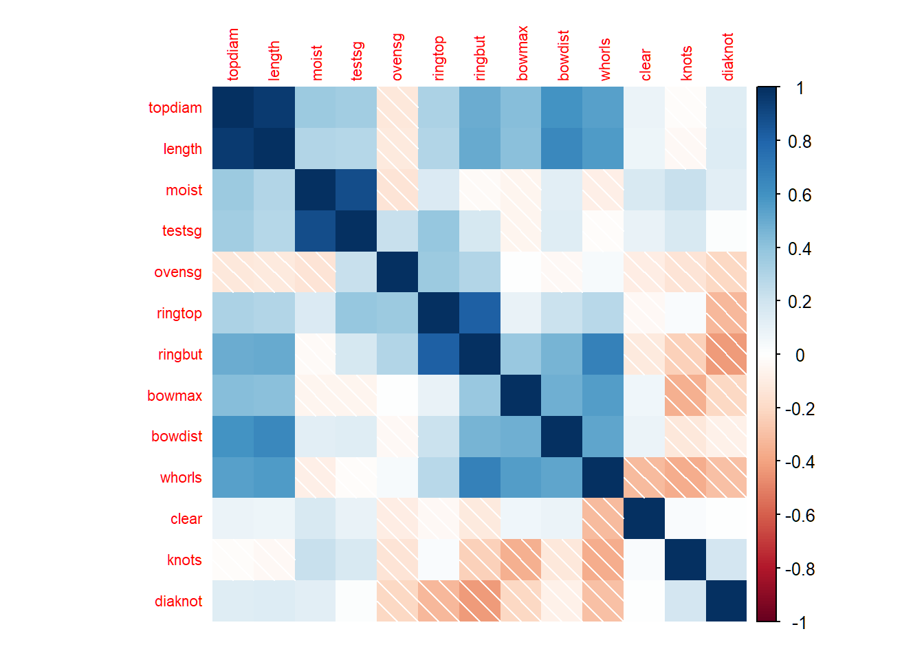

SPCA via tuning parameters

The first 6 sparse PCs are obtained by setting tuning parameters:

> library(elasticnet); data(pitprops)
> out1=elasticnet::spca(pitprops,K=6,type="Gram",
+         sparse="penalty",lambda=1e-6,
+         para=c(0.06,0.16,0.1,0.5,0.5,0.5))
> # loading vectors
> out1$loadings
               PC1         PC2         PC3 PC4 PC5 PC6
topdiam -0.4773598  0.00000000  0.00000000   0   0   0
length  -0.4758876  0.00000000  0.00000000   0   0   0
moist    0.0000000  0.78471386  0.00000000   0   0   0
testsg   0.0000000  0.61935898  0.00000000   0   0   0
ovensg   0.1765675  0.00000000  0.64065264   0   0   0
ringtop  0.0000000  0.00000000  0.58900859   0   0   0
ringbut -0.2504731  0.00000000  0.49233189   0   0   0
bowmax  -0.3440474 -0.02099748  0.00000000   0   0   0
bowdist -0.4163614  0.00000000  0.00000000   0   0   0
whorls  -0.4000254  0.00000000  0.00000000   0   0   0
clear    0.0000000  0.00000000  0.00000000  -1   0   0
knots    0.0000000  0.01333114  0.00000000   0  -1   0
diaknot  0.0000000  0.00000000 -0.01556891   0   0   1
> # adjusted percentage of explained variance
> out1$pev
[1] 0.28034916 0.13965535 0.13298210 0.07444957 0.06801883
[6] 0.06227288

SPCA via sparsity levels

The first 6 sparse PCs are obtained by setting numbers of nonzero entries for sparse loading vectors:

> library(elasticnet); data(pitprops)
> out2<-elasticnet::spca(pitprops,K=6,type="Gram",
+           sparse="varnum",para=c(7,4,4,1,1,1))
> out2$loadings
               PC1         PC2         PC3 PC4 PC5 PC6
topdiam -0.4774878  0.00273577  0.00000000   0   0   0
length  -0.4691409  0.00000000  0.00000000   0   0   0
moist    0.0000000  0.78520583  0.00000000   0   0   0
testsg   0.0000000  0.61854739  0.00000000   0   0   0
ovensg   0.1797963  0.00000000  0.65551907   0   0   0
ringtop  0.0000000  0.00000000  0.58924631   0   0   0
ringbut -0.2898492  0.00000000  0.46990985   0   0   0
bowmax  -0.3425338 -0.02904206 -0.04762634   0   0   0
bowdist -0.4138718  0.00000000  0.00000000   0   0   0
whorls  -0.3833453  0.00000000  0.00000000   0   0   0
clear    0.0000000  0.00000000  0.00000000  -1   0   0
knots    0.0000000  0.00000000  0.00000000   0  -1   0
diaknot  0.0000000  0.00000000  0.00000000   0   0   1
> # adjusted percentage of explained variance
> out2$pev
[1] 0.28171026 0.13933060 0.13067145 0.07439423 0.06845471
[6] 0.06327273

• PC1 loading vector has 7 nonzero entries

Human cancer microarray data

Human cancer data:

• 6830 genes (i.e., \(p=6830\) features) and their expressions
• 64 samples (i.e., \(64\) cancer cell lines)
• 14 different cancer types; information on cancer types at wiki-NCI60

We will pick all genes for 3 caner types “BREAST”, “OVARIAN” and “LEUKEMIA”, and this gives a data matrix \(\mathbf{X} \in \mathbb{R}^{19 \times 6830}\)

SPCA on standardized data

• SPCA will be implemented with tuning parameter \(\lambda=10^{-6}\) for \(l_2\)-penalty and tuning parameters \(\lambda_{1,j}=10^{-6}\) for \(1 \le j \le 18\) for \(l_1\)-penalty

> library(ISLR)
> nci.labs = NCI60$labs; nci.data = NCI60$data
> # pick 3 cancer types: BREAST, OVARIAN, LEUKEMIA
> labs1=nci.labs[nci.labs %in% c('BREAST','OVARIAN','LEUKEMIA')]
> data1=nci.data[nci.labs %in% c('BREAST','OVARIAN','LEUKEMIA'),]
> Xsd = scale(data1,center=TRUE,scale=TRUE)
> # para: amount of l1-penalty if sparse="penalty"
> # lambda: amount of l2-penalty
> # K: number of sparse PCs to be computed
> library(elasticnet)
> resB =elasticnet::spca(Xsd,K=18,para=rep(1e-6,18),
+        type=c("predictor"),sparse=c("penalty"),lambda=1e-6,
+      max.iter=200, eps.conv=1e-3)
> dim(resB$loadings)
[1] 6830   18

First 4 loading vectors

Obtain histograms for first 4 sparse loading vectors:

> library(ggplot2); library(reshape2)
> # the first 4 sparse loading vectors
> FourLD = resB$loadings[,1:4]
> # change column names
> colnames(FourLD) = paste("SPC",1:4,sep="")
> colnames(FourLD)=paste(colnames(FourLD),"loadings",sep=" ")
> # melt and plot
> dstack <- melt(FourLD)
> oLV=ggplot(dstack,aes(x = value))+geom_histogram(bins = 25)+
+   facet_wrap(~Var2,scales="free")+theme_bw()

First 4 sparse loading versions

Histograms for first 4 sparse loading vectors

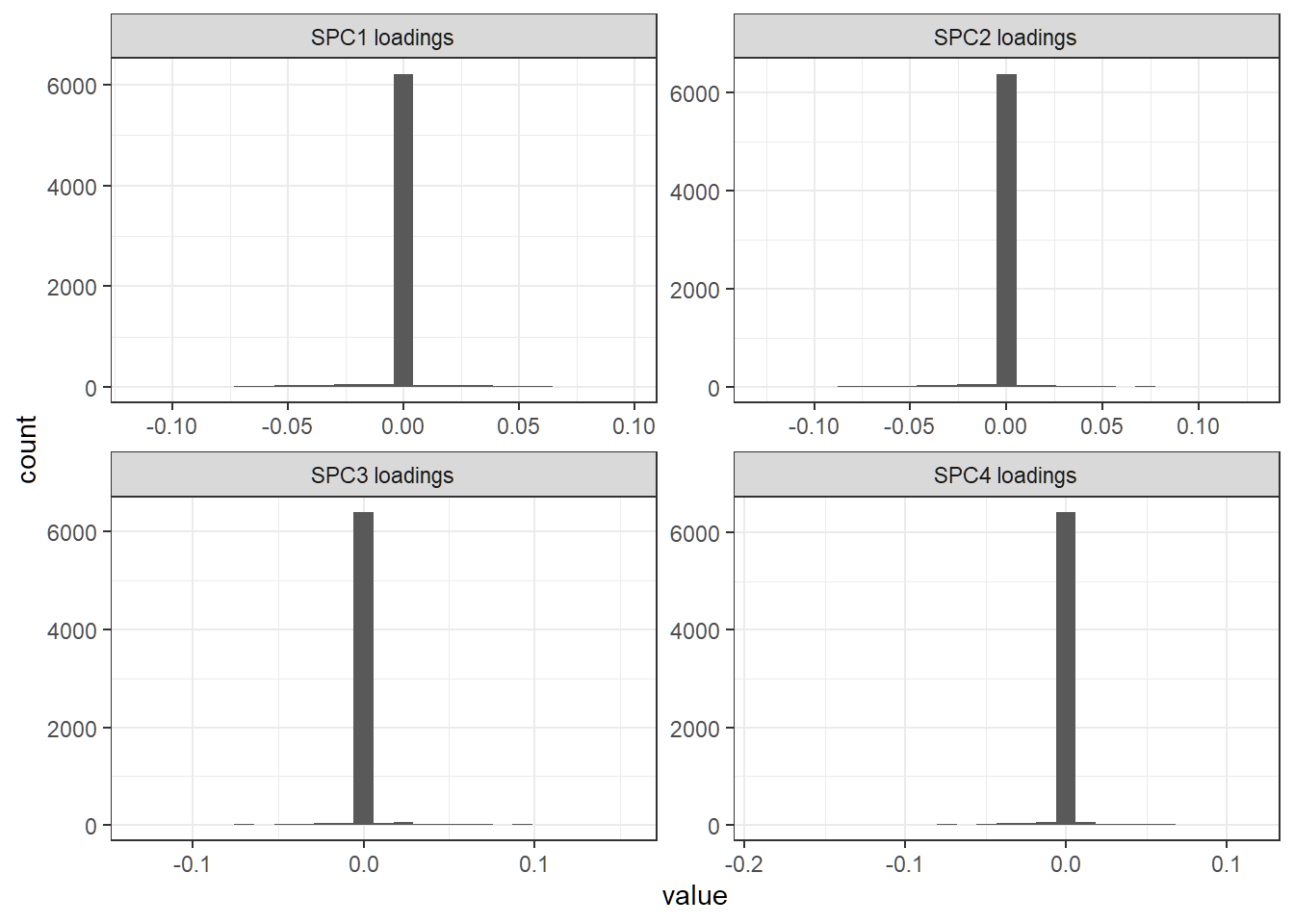
Dominant features

Dominant features (i.e., genes) in sparse direction for SPC1:

> # FourLD has the first 4 sparse loading vectors
> # as its 4 columns
> LV1 = FourLD[,1] # first sparse loading vector
> # all dominant features as those with nonzero loadings
> DF1 = which(abs(LV1)>0)
> length(DF1)
[1] 680
> # dominant features as those with large loadings
> DF2= which(abs(LV1)> 
+             quantile(abs(LV1[abs(LV1)>0]),probs=c(0.95)) )
> length(DF2)
[1] 34

• Features having nonzero or relatively large (in absolute value) loadings for a loading vector are dominant ones in that direction
• Dominant features can be tracked and identified by their indices or variable names

Adjusted PVE and CPVE

> pve=resB$pev  # adjusted PVE; 18 sparse PCs
> # cumsum(pve) # adjusted CPVE
> par(mfrow=c(1,2),mar=c(9,4,1,3),mgp=c(1.8,0.6,0.3))
> plot(pve,type="o",ylab="Adjusted PVE",xlab="Sparse PC",col="blue")
> plot(cumsum(pve),type="o",ylab="Adjusted Cumulative PVE",
+      xlab="Number of first sparse PCs",col="blue")
> abline(h = cumsum(pve)[11], col="red", lty=2)
> abline(v = 11, col="red", lty=2)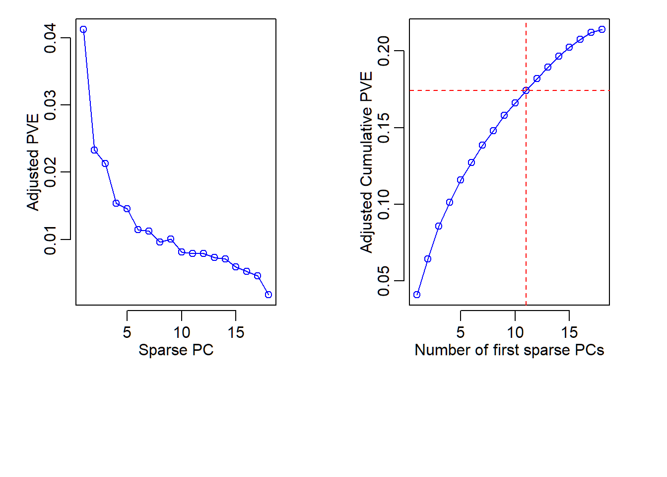

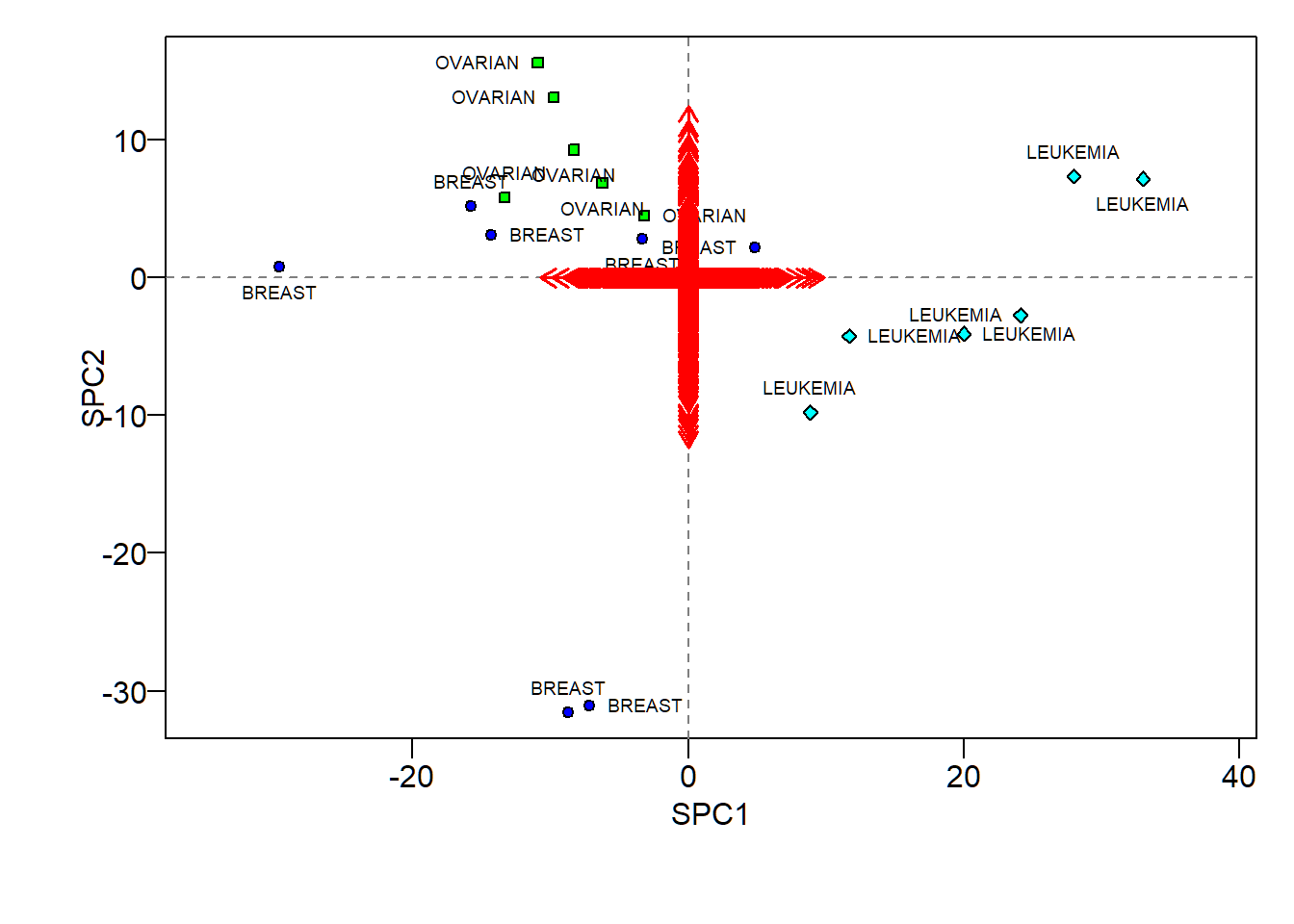
SPCA biplot

Codes to create a biplot for SPCA are bit long but very elementary:

> # get the first 2 loading vectors and score vectors
> sLVTwo=resB$loadings[,1:2]; sSVTwo= Xsd%*%sLVTwo 
> # create color and shape scheme
> pch.group=rep(21,nrow(sSVTwo))
> pch.group[nci.labs1=='BREAST']=21;
> pch.group[nci.labs1=='OVARIAN']=22;
> pch.group[nci.labs1=='LEUKEMIA']=23
> col.group = rep("blue",nrow(sSVTwo))
> col.group[nci.labs1=='BREAST']="blue";
> col.group[nci.labs1=='OVARIAN']="green";
> col.group[nci.labs1=='LEUKEMIA']="cyan"
> # create plot
> par(mar=c(5,4.5,1,1),mgp=c(1.5,0.5,0))
> plot(sSVTwo[,1], sSVTwo[,2], xlab= "SPC1", ylab="SPC2",
+      col="black",pch=pch.group,bg=col.group,
+      las=1,asp=1,cex=0.8)
> # add center lines
> abline(v=0, lty=2, col="grey50")
> abline(h=0, lty=2, col="grey50")
> # add labels
> text(sSVTwo[,1],sSVTwo[,2],labels=nci.labs1,
+      pos=c(1,3,4,2),cex=.6)
> # ending positions of arrows
> l.x=100*sLVTwo[,1]; l.y=100*sLVTwo[,2]
> # draw arrows
> arrows(x0=0, x1=l.x, y0=0, y1=l.y,
+        col="red",length=0.1, lwd=1.5)

SPCA biplot

• Hard to visualize sparse loadings due to too many features
• Scores show some patterns for different cancers (similar to those revealed by ordinary PCA scores)

Caution

library(sparsepca) and library(elasticnet) both implement SPCA but library(sparsepca) may not adjusted PVE

> library(sparsepca)
> # `beta` for l2 penalty and `alpha` for l1 penalty
> resC =sparsepca::spca(Xsd, k=18, alpha=1e-6,beta=1e-6,
+             center=T,scale=T,max_iter=200,
+             tol=1e-05,verbose = FALSE)
> summary(resC)
                            PC1     PC2     PC3     PC4
Explained variance     1157.853 708.803 649.256 499.433
Standard deviations      34.027  26.623  25.481  22.348
Proportion of variance    0.170   0.104   0.095   0.073
Cumulative proportion     0.170   0.273   0.368   0.441
                           PC5     PC6     PC7     PC8     PC9
Explained variance     455.948 390.844 373.202 325.020 323.587
Standard deviations     21.353  19.770  19.318  18.028  17.989
Proportion of variance   0.067   0.057   0.055   0.048   0.047
Cumulative proportion    0.508   0.565   0.620   0.668   0.715
                          PC10    PC11    PC12    PC13    PC14
Explained variance     284.448 272.839 268.269 258.047 245.667
Standard deviations     16.866  16.518  16.379  16.064  15.674
Proportion of variance   0.042   0.040   0.039   0.038   0.036
Cumulative proportion    0.757   0.797   0.836   0.874   0.910
                          PC15    PC16    PC17   PC18
Explained variance     212.511 187.062 156.990 58.830
Standard deviations     14.578  13.677  12.530  7.670
Proportion of variance   0.031   0.027   0.023  0.009
Cumulative proportion    0.941   0.968   0.991  1.000
> # par(mfrow=c(1,2),mar=c(9,4,1,3),mgp=c(1.8,0.6,0.3))
> # plot(1:ncol(sResB),sResB[3,],type="o",ylab="PVE",xlab="Sparse PC",col="blue")
> # plot(sResB[4,],type="o",ylab="Cumulative PVE",xlab="Number of sparse PCs",col="blue")
> # abline(h = cumsum(pve)[11], col="red", lty=2)
> # abline(v = 11, col="red", lty=2)

R software and commands

R libraries and commands needed:

• R library ggbiplot and its command ggbiplot to customize biplot

Command ggbiplot

ggbiplot{ggbiplot} creates a biplot for PCA using ggplot2. Its basic syntax is:

ggbiplot(pcobj, choices = 1:2, scale = 1, pc.biplot =
  TRUE, obs.scale = 1 - scale, var.scale = scale, groups =
  NULL, labels = NULL, labels.size = 3, alpha = 1,
  var.axes = TRUE, varname.size = 3,
  varname.adjust = 1.5, varname.abbrev = FALSE)

• pcobj: an object returned by command prcomp
• choices: which PCs to plot

Command ggbiplot

Basic syntax:

ggbiplot(pcobj, choices = 1:2, scale = 1, pc.biplot =
  TRUE, obs.scale = 1 - scale, var.scale = scale, groups =
  NULL, labels = NULL, labels.size = 3, alpha = 1,
  var.axes = TRUE, varname.size = 3,
  varname.adjust = 1.5, varname.abbrev = FALSE)

• scale: covariance biplot (scale = 1), form biplot (scale = 0). When scale = 1, the inner product between the variables approximates the covariance and the distance between the points approximates the Mahalanobis distance.
• obs.scale: scale factor to apply to observations
• var.scale: scale factor to apply to variables

Command ggbiplot

Basic syntax:

ggbiplot(pcobj, choices = 1:2, scale = 1, pc.biplot =
  TRUE, obs.scale = 1 - scale, var.scale = scale, groups =
  NULL, labels = NULL, labels.size = 3, alpha = 1,
  var.axes = TRUE, varname.size = 3,
  varname.adjust = 1.5, varname.abbrev = FALSE)

• pc.biplot: for compatibility with command biplot.princomp
• groups: optional factor variable indicating the groups that observations belong to. If provided, points will be colored according to groups
• labels: optional vector of labels for the observations
• labels.size: size of the text used for the labels

Command ggbiplot

Basic syntax:

ggbiplot(pcobj, choices = 1:2, scale = 1, pc.biplot =
  TRUE, obs.scale = 1 - scale, var.scale = scale, groups =
  NULL, labels = NULL, labels.size = 3, alpha = 1,
  var.axes = TRUE, varname.size = 3,
  varname.adjust = 1.5, varname.abbrev = FALSE)

• alpha: transparency value for the points (0 = transparent, 1 = opaque)
• var.axes: draw arrows for the variables?
• varname.size and varname.abbrev: size of the text for and whether or not to abbreviate variable names
• varname.adjust: adjustment factor the placement of the variable names; a value >= 1 means farther from the arrow

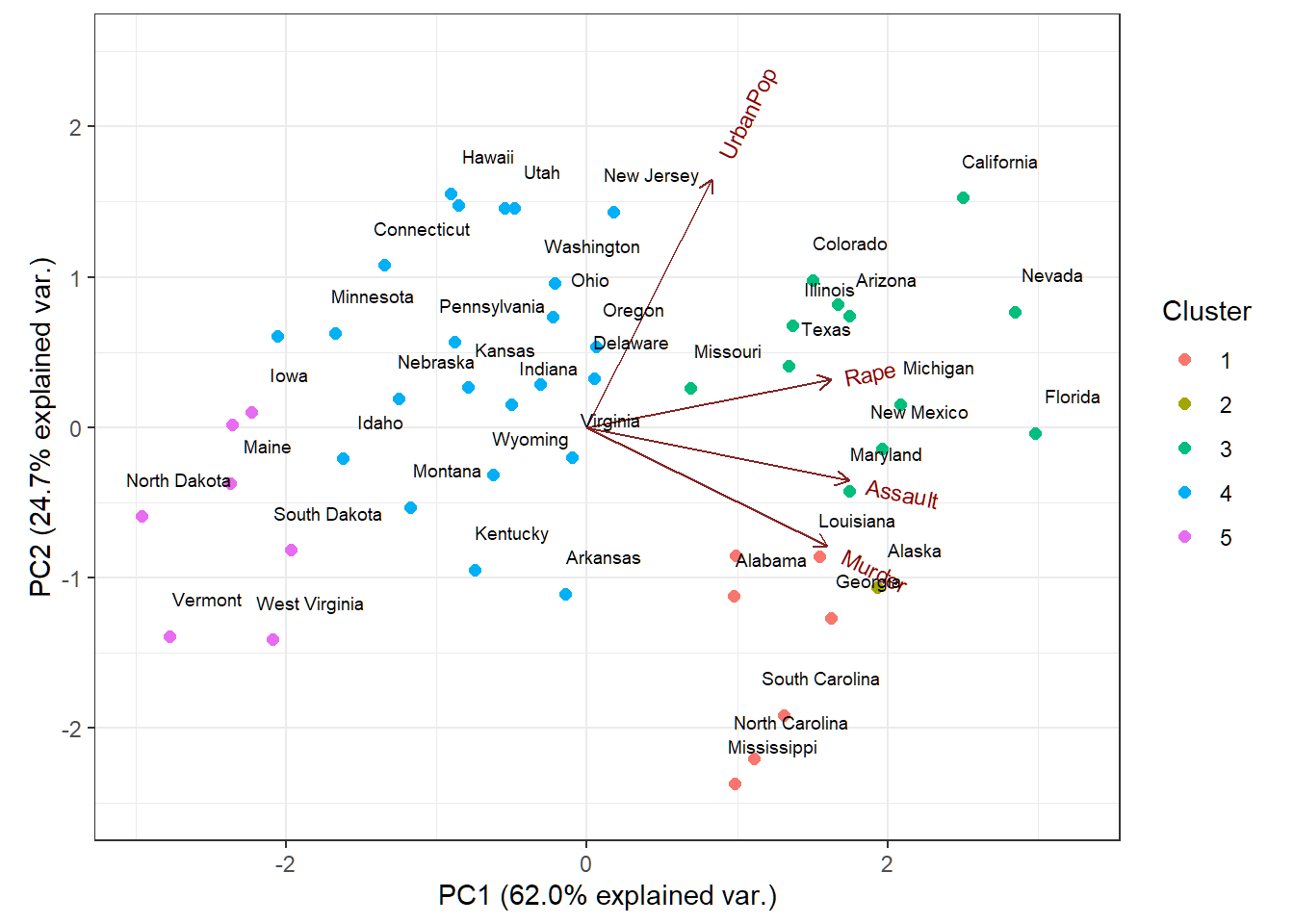
Biplot with clustering

Cluster memberships of US states superimposed on biplot of PCA of USArrests data

> library(ISLR)
> Xsd = scale(USArrests,center=TRUE,scale=TRUE)
> # hierarchical clustering
> hc=hclust(dist(Xsd), "ave"); hc5=cutree(hc, k=5)
> pcaXsd = prcomp(Xsd)
> # change orientation or loading and score vectors
> pcaXsd$rotation= -pcaXsd$rotation; pcaXsd$x= -pcaXsd$x
> # better biplot
> library(ggbiplot)
> cbiF= ggbiplot(pcaXsd,choices=1:2,obs.scale=1,var.scale=1)+
+  geom_point(aes(color=factor(hc5)),size=2)+
+  labs(colour="Cluster",shape="Cluster")+
+ theme(legend.direction = 'horizontal',
+         legend.position = 'top')+ylim(-2.5,2.5)+
+ theme_bw()+geom_text(label=rownames(USArrests), 
+     nudge_x=0.25, nudge_y=0.25, cex=2.5, check_overlap=T)

Biplot with clustering

Cluster memberships superimposed on biplot

Command princomp{stats}

princomp{stats} performs a PCA on a given numeric data matrix and returns the results as an object of class princomp. Its basic syntax is:

princomp(x, cor = FALSE, scores = TRUE, covmat = NULL,
         subset = rep_len(TRUE, nrow(as.matrix(x))),
         fix_sign = TRUE, ...)

• x: a numeric matrix or data frame which provides the data for the principal components analysis.
• cor: a logical value indicating whether the calculation should use the correlation matrix or the covariance matrix. (The correlation matrix can only be used if there are no constant variables.)

Command princomp{stats}

Basic syntax:

princomp(x, cor = FALSE, scores = TRUE, covmat = NULL,
         subset = rep_len(TRUE, nrow(as.matrix(x))),
         fix_sign = TRUE, ...)

• scores: a logical value indicating whether the score on each principal component should be calculated.
• covmat: a covariance matrix, or a covariance list as returned by cov.wt (and cov.mve or cov.mcd from package MASS). If supplied, this is used rather than the covariance matrix of x.

Command princomp{stats}

Basic syntax:

princomp(x, cor = FALSE, scores = TRUE, covmat = NULL,
         subset = rep_len(TRUE, nrow(as.matrix(x))),
         fix_sign = TRUE, ...)

• fix_sign: Should the signs of the loadings and scores be chosen so that the first element of each loading is non-negative? The signs of the columns of the loadings and scores are arbitrary, and so may differ between different programs for PCA, and even between different builds of R: fix_sign=TRUE alleviates that.
• ...: arguments passed to or from other methods. If x is a formula, one might specify cor or scores.

Command princomp{stats}

• princomp is a generic function with “formula” and “default” methods.
• The calculation is done using the command eigen on the correlation or covariance matrix, as determined by cor. A preferred method of calculation is to use svd on x, as is done in prcomp.
• Note that the default calculation uses divisor n (the sample size) for the covariance matrix.
• The print method for these objects prints the results in a nice format, and the plot method produces a scree plot (screeplot). There is also a biplot method.

Command princomp{stats}

princomp returns a list with class “princomp” containing the following components:

• sdev: the standard deviations of the principal components.
• loadings: the matrix of variable loadings (i.e., a matrix whose columns contain the eigenvectors). This is of class “loadings”; see loadings for its print method.
• center: the means that were subtracted.
• scale: the scalings applied to each variable.
• n.obs: the number of observations.

Command princomp{stats}

• scores: if scores=TRUE, the scores of the supplied data on the principal components. These are non-null only if x was supplied, and if covmat was also supplied it was a covariance list. For the formula method, napredict() is applied to handle the treatment of values omitted by the na.action.
• call: the matched call.
• na.action: If relevant.

License and session Information

License

> sessionInfo()
R version 3.5.0 (2018-04-23)
Platform: x86_64-w64-mingw32/x64 (64-bit)
Running under: Windows 10 x64 (build 19041)

Matrix products: default

locale:
[1] LC_COLLATE=English_United States.1252 
[2] LC_CTYPE=English_United States.1252   
[3] LC_MONETARY=English_United States.1252
[4] LC_NUMERIC=C                          
[5] LC_TIME=English_United States.1252    

attached base packages:
[1] stats     graphics  grDevices utils     datasets  methods  
[7] base     

other attached packages:
[1] knitr_1.21

loaded via a namespace (and not attached):
 [1] compiler_3.5.0  magrittr_1.5    tools_3.5.0    
 [4] htmltools_0.3.6 revealjs_0.9    yaml_2.2.0     
 [7] Rcpp_1.0.0      stringi_1.2.4   rmarkdown_1.11 
[10] stringr_1.3.1   xfun_0.4        digest_0.6.18  
[13] evaluate_0.12